Table of Contents
Introduction
LynxKite from Lynx Analytics is a graph analytics platform. It can ingest vast amounts of data, interpret it as huge graphs (aka networks) and enable its users to turn the immense information hidden as billions of network connections into business value.
It does that by providing fast data discovery via innovative visualization options, featuring a rich set of business relevant graph algorithms and facilitating various ways of propagating information via the network connections.
With a distributed architecture powered by Apache Spark, it can scale up to any size of data.
But don’t just believe us — try it! We hope this user guide will be a good companion in your journey of network data mining and you will strike gold for your enterprise with LynxKite!
Hotkeys
For faster navigation you can access certain LynxKite features via hotkeys. The keys available
depend on where you are in the program. You can always see the list of currently available
hotkeys by pressing the ? key.
Workspace browser
The workspace browser is the interface that welcomes you when you navigate to LynxKite in a browser. Like a file browser, it makes it possible to navigate a folder structure and delete or move items. It also allows creating new folders and workspaces — commonly referred to as entries.
To make navigation easier the workspace browser remembers the last folder that was open.
Folders
Folders make it possible to keep the workspaces and other items in LynxKite organized. A common way to
group the items is by user: so the workspaces and snaphots of one user would be in a separate folder from the
workspaces and snapshots of another. This organization is encouraged by assigning a private folder to each user
inside the Users folder.
Click New folder to create a new folder inside the current folder.
Workspaces
Workspaces allow users to describe complex computation flows visually. For a detailed description see the Workspace user interface section.
Click New workspace to create a new, empty workspace inside the current folder. The workspace immediately opens when created and you can start importing data into it.
Access the dropdown menu for a workspace in the workspace browser () to discard, duplicate, or rename the workspace. The rename command also makes it possible to move the workspace to a different path.
Discarding a workspace moves it to the Trash folder in your home folder. This provides means to undo a deletion: just navigate to Trash and move the workspace back to its original location. Discarding a workspace that is already inside Trash deletes it irretrievably. Delete Trash to discard everything inside permanently.
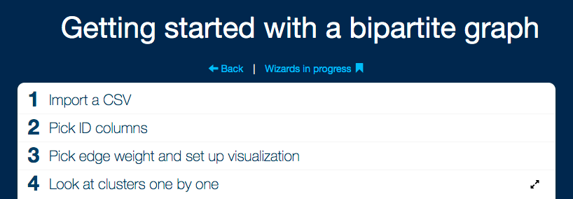
Wizards
Wizards are dedicated tools that distill complex analysis workflows into a series of simple steps. See Authoring wizards to learn how they are created.
Wizards appear in the workspace browser with the icon.
If you click a wizard, a copy will be created in your user directory. This copy is marked as in-progress and its icon changes to . When you click an in-progress wizard, it opens normally and you can continue where you left off.
If you want to edit the workspace behind the wizard, open the dropdown menu in the workspace browser () and choose the Open workspace option.
You can also access the workspace of an in-progress wizard by opening the wizard and clicking the View workspace / Fine tune in workspace button
After opening a wizard, you can fill out the parameters for each step. Click on a heading to move to that step. You can move back or forward as much as you like. Your changes are captured in your "In progress wizards" directory.
Steps with visualizations or large parameter lists benefit from a full-screen view. Click the icon on the current step to switch to maximized view. Click the icon to return to the sequential view.
Snapshots
Snapshots are saved box output states from workspaces. Once a snapshot is saved (see Saving snapshots) it is detached from all workspaces. A snapshot can be of any type that a box output can, such as a graph or a table.
Snapshots can be loaded back into a workspace with an Import snapshot box.
Snapshot content can be viewed inside the workspace browser. Click on the snapshot entry to open/close the snapshot viewer.
Built-ins
The built-ins directory is created by default for every LynxKite instance. It contains
helpful built-in workspaces which can be used as custom boxes. Built-ins are loaded automatically
every time LynxKite restarts and should not be modified directly.
Workspace user interface
A workspace can be opened from the Workspace browser. This section describes the user interface of a workspace.
Workspace header bar
The workspace title bar contains the name of the workspace, its full path (the folders they are in) and buttons to various program functions. It looks something like this:

If the workspace is in the Root folder, it will only show the name of the workspace, as seen above. When you dive into a custom box, the workspace title changes and shows the custom box’s name and path.
Workspace header buttons
Not all the buttons listed here are accessible at all times, please see the details below on when each function is available.
- Save selection as custom box
-
Creates a custom box of the selected boxes. Only available if at least one box is selected. The custom box will be saved under the specified full path. A full path in the LynxKite directory system has the following form:
top_folder/subfolder_1/subfolder_2/…/subfolder_n/name
Keep in mind that there is no leading slash at the beginning of the path. The list of custom boxes, shown on the UI, is limited to special directoriesbuilt-ins,custom_boxes,a/custom_boxes,a/b/custom_boxes,… when we edit the workspacea/b/…/workspace_name. - Save as Python code
-
Generates Python API code for the selected boxes. If nothing is selected, the whole workspace is used.
- Delete selected boxes
-
Removes the selected boxes. Only available if at least one box is selected.
- Dive out of custom box
-
Closes the custom box workspace and returns to the main workspace. Only available if a custom box workspace is opened.
- Dive into custom box
-
Opens the selected custom box as a workspace. Only available if a custom box is selected.
- Select boxes on drag
-
If this mode is enabled, boxes can be selected by dragging a selection rectangle. You can still pan (move the viewport) by clicking and dragging while holding Shift, or select boxes individually (and add boxes to the selection by holding Ctrl).
- Pan workspace on drag
-
If this mode is enabled, clicking and dragging will move the viewport. Boxes can be selected two ways: individually, when additional boxes can be added to the selection by holding Ctrl or by dragging a selection rectangle while holding Shift.
- Undo
-
Undoes the last change performed on the workspace.
- Redo
-
Redoes the last undone change. Only available if you haven’t performed any new changes since the last undo.
- Save workspace as
-
Makes a copy of the current workspace with a new name. You will have write permissions to the new copy even if you did not have for the original.
- Close workspace
-
Closes the workspace.
Boxes and arrows
Workspaces allow users to describe complex computation flows visually by creating workflows represented by boxes and arrows. Boxes represent operations and they are connected by arrows. The sequence of operations applied to the data is shown on a path determined by the arrows.
After creating a new workspace, the viewport is empty, except for the Anchor located in the left
corner. The anchor can be used to explain the overall purpose of the workspace. You can add a
description, an image and set parameters (more details: Parametric parameters). The URL to an
image is useful when you want to reuse the workflow as a custom box in another workspace: in that
case the image will serve as the custom box’s icon. Preferably this should be a link to a local
image, like images/icons/anchor.png.
You can add a box to the workspace by dragging an operation from The operation toolbox. Clicking on the box opens its Box parameters popup, which allows you to set the parameters.
A box can have: inputs (on its left) and outputs (on its right). A box will indicate the number of boxes that can be connected to it and the type of the required input or output (for example: graph, table).
You can add arrows to the viewport by connecting the boxes. Boxes can be connected two ways:
-
Automatically, by hovering the input of one box over the output of another.
-
Manually, by clicking on the output of one box, then dragging the arrow to the input of another.
When two boxes are connected, the computation of the selected operation starts. The color of the output will indicate the status:
-
Red: error, something’s wrong
-
Blue: not yet computed
-
Yellow: currently computing
-
Green: computed
Clicking on the output of a box will open State popups.
Tips & tricks
Instead of clicking on the search bar, you can use the / button. After finding the coveted box,
you can press Enter to place the box under your mouse. You can place multiple boxes without leaving
the search bar.
Boxes and connected box sequences can be copy-pasted, even to different workspaces and LynxKite instances. A limitation here is that the custom boxes are not copied, so they have to be present on the target instance too.
The copy-paste mechanism is implemented via serializing to YAML, a human-readable and editable
textual format, so you can even save box sequences to text files or share them via email. Such
a YAML-file (if it has a .yaml extension) can also simply be drag-and-dropped into a LynxKite workspace.
Hold SHIFT while moving a box to align it to a grid.
Box parameters popup
Clicking on a box opens its box parameters popup. This popup allows you to set the parameters of the box. A faint trail connects the popup to the box it controls. Click the box again, or click on the in the top right corner to close the popup.

Click More about "…" to expand the help page for the box. It can be useful to review the help page when using a box for the first time.
The short description for each parameter can also be accessed by clicking or hovering over the icons by each parameter.
Applying boxes to segmentations
What if you wanted to compute PageRank for the communities in the graph?
If you want to apply a box to a segmentation, first add the box as normal. Then in the box parameters popup adjust the special Apply to parameter to pick the segmentation. This special parameter is added for all graph-typed inputs, making it possible to work with segmentations (and the segmentations of those segmentations, etc.).
Parametric parameters
Parametric parameters can reference workspace parameters.
For example, consider a workspace with two Import CSV boxes, one importing accounts-2017.csv
and the other importing transactions-2017.csv. You could add a workspace parameter called date
with default value 2017. Make the file name parameter of the import boxes parametric by clicking
the icon to the right of the parameter input. Change the file
name parameters to accounts-$date.csv and transactions-$date.csv. Now 2017 will be substituted
for $date, importing the same files as before.
One benefit of this is that you can change the date in a single place (on the anchor box) instead of having to update multiple boxes when the time comes.
Another benefit is that if your workspace is used as a custom box in another workspace, the workspace parameters are specified by the user. Parametric parameters allow you to pass these user-specified parameters on to boxes in the workspace.
Even complex parameters, like a list of vertex attributes, can be toggled to become parametric. In this case the original input field is replaced by a simple text field.
Parametric parameters are evaluated using
Scala string interpolation.
This means that Scala expressions can be embedded in these parameters. For example, you could write
accounts-${date.toInt + 1}.csv.
Built-ins in parametric parameters
Besides the workspace parameters, a few built-in values are also accessible in parametric parameters to help implement flexible solutions.
vertexAttributes, edgeAttributes, and graphAttributes are lists of objects
with name and typeName properties corresponding to the attributes found on the graph
inputs of the box. They could be used, for example, to convert all string attributes to
numbers with a Convert vertex attribute to number box. Manually selecting the
attributes only works for a fixed input. But all inputs can be covered with a parametric
parameter:
${
  vertexAttributes
    .filter(_.typeName == "String")
    .map(_.name)
    .mkString(",")
}
workspaceName is only available in a top-level workspace, and not inside custom boxes.
It holds the name of the workspace as a string. One use case for this is in
wizards. Opening a wizard will create a copy of it, which will have
a new, unique workspace name. Using this workspace name in a parametric parameter can
ensure that the parameter has a unique value. For example, if your Create graph in Python
box uses randomness or an external data source, you can force its re-evaluation by
making the code a parametric parameter and including the workspace name in a comment.
# $workspaceName
import random
...
Unexpected parameters
Unexpected parameters are parameters that have been set at some point on the box, but are no longer recognized.
The list of parameters for many boxes is determined dynamically. For example in
Aggregate on neighbors there is one parameter for each vertex attribute. If you have configured
an aggregation for attribute X but then changed the input to no longer have an attribute called
X, then the parameter that sets aggregation on X becomes an unexpected parameter.
Unexpected parameters are treated as errors. You can click the icon to the right to remove the unexpected parameter. Or you can change the input so that the parameter becomes recognized again.
Box metadata
Click the icon in the popup header to access the box metadata. Click the icon to return to the parameter editor.

- Box ID
-
The internal identifier of this box within the workspace. This is only visible when storing the box in a text format.
- Operation
-
The operation that this box represents. You can edit this to change the type of the box. For example you could turn an Import CSV box into an Import Parquet box.
State popups
Click on an output of a box to open that output state in a popup. Click the output again, or click on the icon in the top right corner to close the popup. You can also press ESC to close the last used popup.
Different output types have different data and features available in their popups. But some things they all have in common.
Saving snapshots
The toolbar at the top of the state popup always contains a icon, for saving the state as a snapshot. The snapshot will be saved outside of the workspace, in the directory tree. Snapshots are independent of the workspaces from which they were saved. Use them to share final results, or record intermediate results for comparison.
To save a snapshot you have to specify the full path of the snapshot.
A full path in the LynxKite directory system has the following form:
top_folder/subfolder_1/subfolder_2/…/subfolder_n/name
Keep in mind that there is no leading slash at the beginning of the path.
Snapshots can be loaded back into a workspace with an Import snapshot box.
Instruments
Boxes like Graph visualization, SQL1, Custom plot are essential for looking at your data. It is very natural to want to take a quick look at the data in the middle of a complex workspace.
One option is to quickly create and attach a Graph visualization box, see what the graph looks like at that point, and then delete the box. Instruments are effectively the same, except that no temporary box is added to the workspace. This means instruments can be used even on read-only workspaces.
The instrument buttons are in the popup toolbar. For example, in the last screenshot the buttons for SQL and Visualize are visible, corresponding to the SQL1 and Graph visualization boxes. If you click on SQL, the popup contents are replaced by the box parameters of the SQL1 box at the top and the output state of the SQL1 box at the bottom.
The output state of the instrument once again has a toolbar for snapshotting and applying instruments. This makes it possible to apply one instrument after the other:
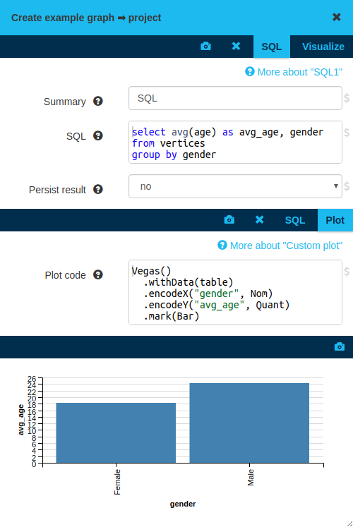
Instruments are not saved into the workspace. But they are built from regular boxes, so the same calculations can always be reproduced using conventional boxes.
Graph state
We use the word graph for a rich type that represents the base graph and its segmentations in one bundle. The popup for a graph shows basic information about the base graph, such as the number of vertices and edges. It lists the attributes and segmentations. Graph attribute values are displayed, attribute histograms are available on click, and segmentations can be opened to dig deeper.
The Graphs chapter gives a more in-depth description of graphs.
Table state
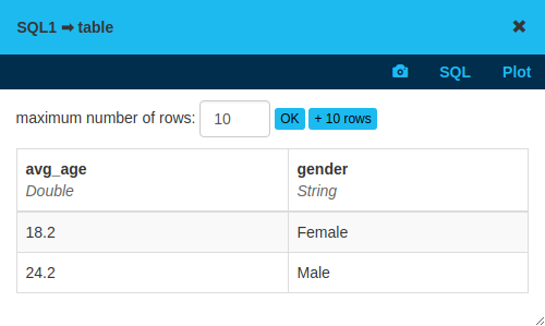
Tables are the same in LynxKite as in relational databases and spreadsheet programs: they are a matrix of columns and rows. Tables are the input and output of SQL queries. Graphs can be built from tables via Use table as vertices, Use table as edges, and similar operations.
Plot state
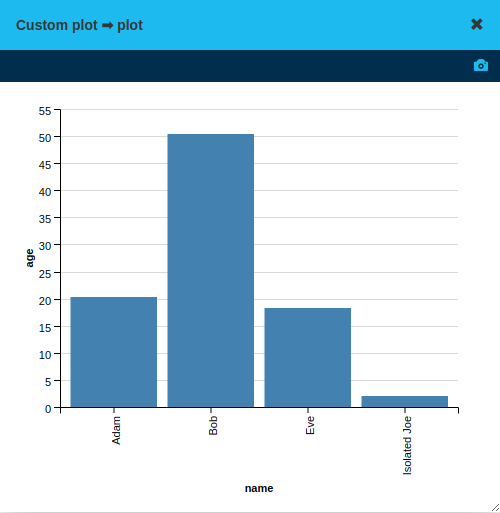
The plot state is a data visualization created via the Custom plot box, or one of the built-in plotting boxes.
Export state
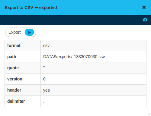
Export boxes, such as Export to CSV, allow you to configure an export operation. The output of these boxes is an export state. It is the export state which actually allows triggering the often resource-intensive computation of creating the output files.
This two-step process avoids accidental exports while editing the workspace. It also provides metadata information about the output, for example a file path. To trigger the export, click on the icon.
Custom boxes
It is easy to extend LynxKite with custom boxes that are specific to a project or organization. Wrapping logical parts of your workspaces in custom boxes makes the workspace easier to understand and avoids repetition.
A custom box is simply another workspace. If you place a workspace in the X/Y/custom_boxes
directory, you will be able to use it as a custom box in any workspaces recursively under X/Y.
If you place a workspace in the top-level custom_boxes directory, any workspace in this LynxKite
instance will be able to use it. This system of scoping makes it possible to organize
project-specific or universally useful custom boxes.
If you place a workspace in custom_boxes, it will appear in the box catalog under the
"Custom boxes" category, and in the box search. You can place it in a workspace.
A usual workspace used this way will result in a custom box that has no inputs and outputs. That is not very useful! To fix that, just add Input and Output boxes to the workspace of the custom box.
It is inconvenient to work with Input boxes, because their output is missing. It will be filled in when the custom box is used in another workspace. But when you’re editing the workspace of the custom box directly, there is nothing coming in yet. There are two solutions to this:
-
Place your custom box in a workspace. Connect its inputs. Select it and dive into the custom box with the button. Now you will see and edit the workspace of the custom box in the context of the parent workspace. The input box will have a valid output: the state that is coming in from the parent workspace.
Any changes you make will affect all instances of the custom box.
-
It is often the case that your workspace grows and you reach a point where you want to extract part of it into a custom box. Do not create a workspace in
custom_boxesmanually in this case. It is simpler to select the part of the workspace that you want to wrap into a custom box and click the Save selection as custom box button instead.The workspaces of custom boxes created this way will automatically have the input and output boxes set up.
Custom box parameters
Your custom box now has inputs and outputs and can provide useful functionality. Custom boxes can also take parameters. This is configured through the Anchor box of the workspace of the custom box.
You can set the name, type, and default value of the parameters. The following parameter types are supported:
-
Text: Anything that the user can type. It could be a string or a number. This will appear as a plain input box in the custom box’s parameters popup.
-
Boolean: Will appear as a true/false dropdown selection in the box parameters popup.
-
Code: Will appear as a multi-line code editor to the user.
-
Choice: Will appear as a dropdown list. List the offered options after the default value, separated by a comma.
-
Vertex attribute, edge attribute, graph attribute, segmentation, column: These types allow the user to select an attribute, segmentation, or column of the input via a dropdown list. If the custom box has multiple inputs, the options belonging to all the inputs will be offered in the list.
To make use of the custom box’s parameters in the workspace of the custom box, you need to access
them from Parametric parameters. Regardless of their type, all the parameters are seen as
Strings from the Scala code of the parametric parameters. Use .toInt, .toDouble, .toBoolean
on them if you need to do more than simple string substitution.
Authoring wizards
You can build complex analysis workflows in LynxKite workspaces. You can encapsulate such workflows in Custom boxes so that other LynxKite users can reuse them. Another way to share your work is in the form of wizards.
To turn a workspace into a wizard, open the parameters of the Anchor box and set the Wizard parameter to yes. Now your workspace is a wizard. But it doesn’t have any steps yet.
Each step in a wizard corresponds to a parameter or state popup from the workspace. There are two ways to add steps to the wizard. The anchor box has a table of steps:
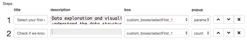
In this table you can specify:
-
The title of the step. This appears on the wizard view in a large font.
-
The description of the step. This is a multi-line field where you can add more text to the step using Markdown syntax. This makes it possible to use formatted text with images and links.
-
The box from which you want to use the parameter or output state.
-
The popup column lets you choose "parameters" (to use the parameter popup) or one of the output states of the box.
-
The order of the steps using the buttons on the right. Press or to move the step up or down, or to delete the step.
You can also quickly add steps to a wizard from a parameter or state popup. Once the workspace is configured as a wizard, each popup will have a icon in the header bar. Click this icon to add or remove the popup as a step.
Using custom boxes as steps in a wizard makes it possible to create interfaces specially crafted for a specific use case.
Using wizards
Once a workspace has been configured as a wizard, clicking it in the workspace browser takes you to the wizard view.
If the In progress setting is disabled in the Anchor box, opening the wizard creates a copy of it. This way multiple users can work off of the same wizard without interfering with each other. The copies will be created with the In progress setting enabled. Opening these copies then will not create further copies.
See our section on Wizards in the workspace browser for more about how wizards look from outside of the workspace.
Scala guide
You can derive attributes in LynxKite by implementing the derivation formulas using Scala. For a general introduction to the Scala language, see the Tour of Scala.
Getting started
The simplest way of using Scala to derive attributes is to just provide a one-liner expression in Derive vertex attribute or Derive edge attribute. The examples below are for deriving vertex attributes. The only difference from deriving edge attributes is the way vertex attributes can be accessed.
A simple example:
6.0 * 7.0will generate a constant numeric attribute of value 42.0. You can also use values of other attributes
in the expression:
6.0 * ageassuming that there is already an age attribute defined. LynxKite can also accept a list of
Scala expressions:
val x = age + 1.0
val y = num_friends + 2.0
y / x
In this case, the value of the last expression will be taken as the value of the derived attribute. More complex code can be structured using functions:
def getAge() {
  age + 1.0
}
def getNumFriends() {
  num_friends + 2.0
}
getNumFriends() / getAge()
Allowed types
LynxKite uses Scala data types internally, so there is no need for type conversion between LynxKite and the derivations script. However, to support persistence, the available types for both input (the type of vertex and edge attributes the script can use) and result are restricted to the following.
-
Double -
String -
Int(will be automatically converted toDouble) -
Long(will be automatically converted toDouble) -
Vector[X]whereXis a supported type -
(X, Y)whereXandYare supported types
Values of other types need to be manually converted before returning from the Scala script. For input types, you can use, for example, either of Convert vertex attribute to String or Convert vertex attribute to number.
Apache Spark status
LynxKite uses Apache Spark as its distributed computation backend. The status of the backend is reflected by the elements in the bottom right corner of the page.
A single LynxKite operation is often performed as a sequence of multiple Spark stages. A single Spark stage is further subdivided into Spark tasks. Tasks are the smallest unit of work. Each task is assigned to one of the machines in the cluster.
The rotating cogwheel in the bottom right indicates that Spark is calculating something.
The Stop calculation button appears when you hover over the cogwheel. It sends an interruption signal to Spark. This signal aborts work on all Spark stages. The tasks that are in progress will still be finished, but the outstanding tasks and stages will be cancelled. The button cancels all Spark stages, not just the ones initiated by the user pressing the button. For this reason the button is restricted to admin users.
The little colorful rectangles represent Spark stages. The height of the rectangle indicates the percentage of tasks completed in the stage. The color corresponds to the type of work it does.
Graphs
We use the word graph for a rich box output type that represents the base graph and its segmentations in one bundle. The state popup for a graph shows basic information about the base graph, such as the number of vertices and edges. It lists the attributes and segmentations. Graph attribute values are displayed, attribute histograms are available on click, and segmentations can be opened to dig deeper.
Vertex and edge attributes
Vertex attributes are values that are defined on some or all individual vertices of the graph. Edge attributes are values that are defined on some or all individual edges of the graph.
Each attribute has a type. For each vertex/edge the attribute is either undefined or the value of the attribute is a value from the attribute’s type.
Clicking on a vertex or edge attribute opens a menu with the for following information/controls.
-
The type of the attribute (e.g.
String,number, …). -
A short description of how the attribute was created, if available, with link to a relevant help page.
-
A histogram of the attribute, if the attribute is already computed. A menu item to compute the histogram otherwise. By default, for performance reasons, histograms are only computed on a sample of all the available data. Click the "precise" checkbox to request a computation using all the data. Click the "logarithmic" checkbox, to use a logarithmic X-axis with logarithmic buckets. (Useful when the distribution is strongly skewed.)
-
If you are viewing the graph in a Graph visualization box: Controls for adding the attribute
-
to the current visualization, if Concrete vertices view or Bucketed view is enabled. See details in Concrete visualization options.
There are lots of ways you can create attributes:
-
When importing vertices/edges from a CSV every column will automatically become an attribute.
-
You can also import attributes for existing vertices from a CSV file.
-
You can compute various graph metrics on the vertices/edges. (Just to name a few, you can compute Compute degree, Compute clustering coefficient for vertices and Compute dispersion for edges.)
-
You can derive more attributes from existing ones using the Derive vertex attribute and Derive edge attribute operations.
-
You can spread attributes via edges in various ways, e.g. by Aggregate on neighbors.
Undefined values
Sometimes a vertex (or an edge) does not have any value for a particular attribute. For example, in a Facebook graph, the user’s hometown might or might not be given. In such a case, we say that this attribute is undefined for that particular vertex (or edge). Usually, an undefined value represents the fact that the information is unknown.
Note that an empty string and an undefined value are two different concepts.
Suppose, for example, that a person’s name is represented by three attributes:
FirstName, MiddleName, and LastName. In this case, MiddleName could be the
empty string (meaning that the person in question has no middle name), or it could be
undefined (meaning that their middle name is not known). Thus, the empty string is
treated as an ordinary String attribute.
Differences between undefined and defined values:
-
In histograms, undefined values are not counted, whereas defined values (including the empty string) are counted.
-
Filters work only on defined attributes. (See Filter by attributes.)
-
Derive edge attribute and Derive vertex attribute allow you to choose whether to evaluate the expression if some of the inputs are undefined.
Fill vertex attributes with constant default values can be used to replace undefined values with a constant. By replacing them with a special value, they can be made part of histograms or filters.
CSV export/import and undefined
When exporting attributes, LynxKite differentiates between undefined attributes and
empty strings. For example, if attribute attr is undefined for Adam and Eve, but
is defined to be the empty string for Bob and Joe, here’s what the output looks like.
Note that the empty string is denoted by "", whereas the undefined value is
completely empty (i.e., there is nothing between the commas):
"name","attr","age"
"Adam",,20.3
"Eve",,18.2
"Bob","",50.3
"Joe","",2.0
Note, however, that importing this data from a CSV file will treat undefined values
as empty strings. So, in this case, the distinction between undefined values
and empty strings is lost. One way to overcome this difficulty is to replace
empty strings with another, unique string (e.g., "@") before exporting
to CSV files. (Other export and import formats do not suffer from this limitation.)
Creating undefined values
It might be necessary to create attributes that are undefined for certain vertices/edges. (An example use case is when you want to create input for a fingerprinting operation.) This can be done with Derive vertex attribute (or Derive edge attribute) operation. For example, the Scala expression
if (attr > 0) Some(attr) else None
will return attr whenever its value is positive, and undefined otherwise.
Graph attributes
Graph attributes are data that correspond to the whole graph.
For example, you can compute the average of any numeric vertex attribute with Aggregate vertex attribute globally. This average will show up as a graph attribute in the output graph.
Segmentations
The segmentation of a graph is another graph. The vertices of the segmentation are also called "segments". A set of edges exists between the base graph and its segmentation, representing membership in a segment. (To distinguish these special edges we also call them "links".)
For example the Find maximal cliques operation creates a new segmentation, in which each segment represents a clique in the base graph. Vertices of the base graph are linked to the segments which represent cliques that they belong to.
Segmentations serve as the foundation of many advanced operations. For example the average age for each clique can be calculated using the Aggregate to segmentation operation and the average size of the cliques that a person belongs to can be calculated with Aggregate from segmentation.
Segmentations can be opened on the right hand side by clicking them and choosing "Open" in the menu. They can be visualized the usual way. The links are displayed when both the base graph and its segmentation are visualized. This works when both sides are visualized as bucketed graphs, when they are visualized as concrete vertices, or even when one side is bucketed and the other is concrete. This can be used to gain unique insights about the structure of relationships in the graph.
Segmentations act much like the base graph, and you can even import existing graphs to act as segmentations. (In this case it is possible that the links will represent a relationship other than membership.)
Machine learning models
Machine learning models are stored as graph attributes. They are created by a machine learning operation (for example Train linear regression model) and used for prediction with the Predict with model operation or for classification with the Classify with model operation.
Press the plus button () to access detailed information about a machine learning model.
Method
The machine learning algorithm used to create this model.
Label
The name of the attribute that this model is trained to predict. (The dependent variable.)
This will not appear for unsupervised machine learning models.
Scaling
Details about the pre-processing scaling step applied to the features before training. The two phases are centering and scaling. The first phase (centering) centers the data with mean before scaling, i.e., the mean is subtracted from all elements. The data set acquired this way has a mean of 0. The second phase (scaling) is acquired by dividing all the elements by the standard deviation. The means and deviations in these steps are computed columnwise.
Suppose we have an original data item (a, b). After these two steps, the data item that is used for the training will be ((a-m1)/d1, (b-m2)/d2), where m1 and d1 are the mean and the standard deviation for the first column (the a’s) and m2 and d2 are the mean and the standard deviation for the second column (the b’s).
Note that both steps are optional: it depends on the model, whether they are applied or not.
Features
The list of the feature attributes that this model uses for predictions. (The independent variables.)
Details
For decision tree classification model:
-
The i-th element of
supportis the number of occurrences of the i-th class in the training data divided by the size of the training data.
For linear regression and logistic regression models:
-
interceptis the constant parameter in the regression equation of the model. -
coefficientsare the coefficients in the regression equation of the model.
For linear regression model:
-
R-squaredis the coefficient of determination, an index of the linear correlation between the features and the label. -
MAPEis the mean absolute percentage error, a measure of prediction accuracy. -
T-valuescan be used for the hypothesis test of coefficient significances. This will not appear for the lasso model.
For logistic regression model:
-
Z-valuescan be used for the hypothesis test of coefficient significances. -
pseudo R-squared, or McFadden’s R-squared in our case, is an index of the logistic correlation between the features and the label. -
thresholdis the probability threshold for binary classification. If the outcome probability of the label 1.0 is greater than the threshold, the model will predict the classification label as 1.0. The threshold is obtained by maximizing the F-score. -
F-scoreis a measure of test accuracy for binary classifications.
For KMeans clustering model:
-
cluster centersare the vectors of the KMeans cluster centers. -
costis the k-means cost (sum of squared distances of points to their nearest center) for this model on the training data.
Graph visualizations
You can create graph visualizations by adding the operation Graph visualization to your workflows or by clicking on the "Visualize" button in the State popups.
There are multiple types of graph visualizations, but in every case you see some objects connected by some arcs. You can choose to open the Concrete vertices view or the Bucketed view.
Visualized objects can represent vertices or groups of vertices of the graph. The same way arcs on the screen might represent multiple edges in the graph. E.g. if there are multiple parallel edges A → B it will still be represented by a single visualized arc. Also, when we display groups of vertices then a single arc going from one group to another represents all the edges in the graph going from one group to the other.
You can visualize graph attributes in various ways, see details in section Concrete visualization options.
Regardless of the visualization mode you can do the same basic adjustments on the visualization screen:
- Zooming in/out
-
Use your mouse wheel or scroll gesture to zoom in and out. Left double-click and right double-click can also be used for this.
- Panning
-
Hold down your left mouse button anywhere on the visualization screen and drag the graph around.
- Zooming objects in/out
-
Hold down the Shift button while zooming in and out to only change the size of objects (vertices, edges).
Concrete vertices view
Shows some selected center vertices and their neighborhood with all the edges among these vertices. The set of the center vertices and the size of the neighborhood can be selected by the user.
The first line shows the "Visualization settings":
- Display
-
The first button lets you select between 2D and 3D visualization. 3D allows for showing more vertices efficiently but that mode has less features. You cannot (yet) visualize attributes in 3D mode and cannot select and move around vertices.
- Layout animation
-
(Only in 2D mode) If the second button is enabled, layout animation will continuously do a physical simulation on the displayed graph as if edges were springs. You can move vertices around and the graph will reorganize itself.
- Label attraction
-
When animation is enabled, this will make vertices with the same label attract each other, which results in same label vertices being grouped together.
- Layout style
-
When animation is enabled, this option determines the exact physics of the simulation. The different options can be useful depending on the structure of the network that is visualized.
The available options are:
- Expanded
-
Try to expand the graph as much as possible.
- Centralized
-
High-degree nodes in the center, low-degree nodes on the periphery.
- Decentralized
-
Low-degree nodes in the center, high-degree nodes on the periphery.
- Neutral
-
Degree is not factored into the layout.
- Centers
-
Lists "center" vertex IDs, that is the vertices whose neighborhood we are displaying. You can change this list manually, using the Pick button.
- Radius
-
You can set the neighborhood radius from 0 to 10. 0 means center vertices only. 1 means center vertices and their immediate neighbors. 2 also contains neighbors of neighbors. And so on.
- Edge style
-
Edges can either be displayed as directed (the default) or undirected. The directed mode shows edges as curved arrows. In the undirected mode they are displayed as straight lines.
Pick button
This button is used to select a new set of centers. The vertices placed there will be ones that satisfy all the currently set restrictions (see below). The available options are:
- Center count
-
The number of centers to be picked. (Default: 1)
Restrictions narrow down the potential set of candidates that will be chosen when you click on the Pick button. They have the same syntax as filters. (See Filter by attributes.) There are two ways to specify them:
- Use graph attribute filters
-
(Default.) Use the currently set vertex attribute filters as restrictions.
- Use custom restrictions
-
Manually enter restrictions. When switching to this mode, the graph filters are automatically copied into the custom restriction list, which can be edited then.
After picking one set of centers with the Pick button the button is replaced by the Next button. Clicking this button will iterate over samples that match the conditions. The samples will show up in a deterministic order. You can skip to an arbitrary sample by clicking on the button. There you can manually enter a position in the sequence and pick it by clicking on Pick by offset.
Concrete visualization options
Vertex visualizations
- Label
-
Shows the value of the attribute as a label on the displayed vertices.
- Color
-
Colors vertices based on this attribute. A different color will be selected for each value of the attribute. If the attribute is numeric, the selected color will be a continuous function of the attribute value. This is available for
Stringandnumberattributes. - Opacity
-
Changes the opacity of vertices based on this attribute. The higher the value of the attribute the more opaque the vertex will get.
- Icon
-
Displays each vertex by an icon based on the value of this attribute. The available icons are "circle", "square", "hexagon", "female", "male", "person", "phone", "home", "triangle", "pentagon", "star", "sim", "radio". If the value of the attribute is one of the above strings, then the corresponding icon will be selected. For other values we select arbitrary icons. When we run out of icons, we fall back to circle. This is only available for
Stringattributes. - Image
-
Interprets the value of the attribute as an image URL and displays the referenced image in place of the vertex. This can be used e.g. to show facebook profile pictures.
- Size
-
The size of vertices will be set based on this attribute. Only available for numeric attributes.
- Position
-
Available on attributes of type
Vector[number]. The first two elements of the vector will be interpreted as (X, Y) coordinates on the plane and vertices will be laid out on the screen based on these coordinates. (You can create aVector[number]from two number attributes using the Bundle vertex attributes into a Vector operation.) - Geo coordinates
-
Available on attributes of type
Vector[number]. The first two elements of the vector will be interpreted as latitude-longitude coordinates and vertices will be put on a world map based on these coordinates. (You can create aVector[number]from two number attributes using the Bundle vertex attributes into a Vector operation.) - Slider
-
Available for
numberattributes. Adds an interactive slider to the visualization. As you move the slider from the minimum to the maximum value of the attribute, the vertices change their color. Vertices below the selected value get the first color, vertices above the selected value get the second color.You can choose the color scheme to use. If you choose a color scheme where vertices can become transparent, the edges of the transparent vertices will also disappear. This is a great option for visualizing the evolution of a graph over time.
Edge visualizations
- Edge label
-
Will show the value of the attribute as a label on each edge.
- Edge color
-
Will color edges based on this attribute. A different color will be selected for each value of the attribute. If the attribute is numeric, the selected color will be a continuous function of the attribute value. Coloring is available for
Stringandnumberattributes. - Width
-
The width of edge will be set based on this attribute. Only available for numeric attributes.
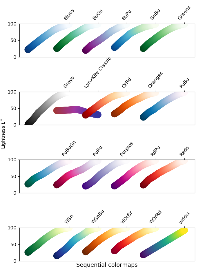
Color maps
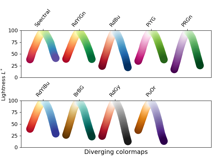
When an attribute is visualized as Vertex color, Label color, or Edge color, you can also choose a color map in the same menu. LynxKite offers a wide choice of sequential and divergent color maps. Divergent color maps will have their neutral color assigned to zero values, while sequential color maps simply span from the minimal value to the maximal.
Lightness is an important property of color maps. A good color map is as linear as possible in lightness charts. For more discussion see Matplotlib’s Choosing Colormaps article.
Lightness charts for the available color maps:
Bucketed view
Shows a consolidated view of all the vertices of the graph. Vertices can be grouped by up to two attributes and the system visualizes the sizes of the groups and the amount of edges going among the groups.
To add a vertex attribute to the visualization, click the attribute and pick "Visualize as" X or Y.
For String attributes, the created buckets will correspond to the possible values of the
attribute.
If the attribute has more possible values than the number of buckets selected by the user then the
program will show buckets for the most frequent values and creates an extra Other bucket for the
rest.
For number attributes buckets will correspond to intervals. We split the interval [min, max]
(where min and max are the minimum and maximum values of the attribute respectively)
into subintervals of the same length. E.g. we might end up with buckets [0, 10),
[10, 20), [20, 30].
If logarithmic mode is selected for the attribute then the subintervals are
selected so that they have the same length on the logarithmic scale. E.g. a possible
bucketing is [1, 2), [2, 4), [4, 8]. In logarithmic mode, if the attribute has any
non-positive values, then an extra bucket will be created which will contain all non-positive values.
Edge attributes can also be added to the visualization to be used for calculating the width of the aggregate edges.
By default the visualization has 4×4 buckets, but this can be adjusted in the visualization settings list.
Relative edge density
Bucketed view by default comes in absolute edge density mode. Absolute edge density means the thickness of an edge going from bucket A to bucket B corresponds to the number of edges going from a vertex in bucket A to a vertex in bucket B (or in the weighted case: to the sum of the weights on such edges). This makes the edges going between large buckets typically much thicker than those going between smaller buckets.
Relative edge density, on the other hand, is calculated by dividing the number of edges between bucket A and bucket B by [size of bucket A] × [size of bucket B]. This way, the individual bucket sizes aren’t reflected on the thickness of the edges.
Precise and approximate counts
For very large graphs the bucketed view numbers are extrapolated from a sample. Precise calculation would not produce a visible change in the visualization, so most often it is not necessary. It can be desirable however if the numbers from the visualization are to be used in a report.
Click the "approximate counts" option to switch it to "precise counts".
Color customization
A color customization panel is accessible in visualizations. Click on the white tab on the left to access the panel.
The panel allows you to copy the visualized data to the clipboard () and customize the color settings. You can invert the colors, increase or decrease brightness (), contrast (), and saturation (). For geographic visualizations the same settings can be applied separately to the map background.
Ray tracing
LynxKite has an optional feature for generating ray traced graph visualizations. These visualizations can give simple graphs a more striking look in presentations and marketing materials.
To enable ray tracing the administrator has to install POV-Ray
and the graphray Python package found in the tools directory of the LynxKite installation.
Open a graph visualization and click  to get a relatively
quick draft render. If you are
satisfied with the layout, click "Render in high quality" to get the final render. Right-click the
final image to save it locally.
to get a relatively
quick draft render. If you are
satisfied with the layout, click "Render in high quality" to get the final render. Right-click the
final image to save it locally.
Ray tracing supports the following visualization features:
-
Vertex colors.
-
Vertex sizes.
-
Highlighting of center vertex.
-
Vertex shapes are translated to simpler 3D shapes.
-
The relative layout and scaling will be reproduced exactly. Only the camera positioning is different.
The rendered image is generated to match the width and height of the popup. Make the popup smaller for faster render times, or larger for higher resolution. The generated picture has a transparent background.
LynxKite internals
Prefixed paths
LynxKite provides read and write access to distributed file systems for the purpose of importing and exporting data. To make this access secure and convenient, paths are specified relative to prefixes.
Prefixes are configured during LynxKite deployment through the prefix_definitions.txt file.
For example, let’s say we want to import a file on Amazon S3. The file is in bucket my-company,
at data/file.csv. The full Hadoop path to this file would be:
s3n://<key id>:<secret key>@my-company/data/file.csv
During deployment, the COMPANY_S3 prefix has been configured:
COMPANY_S3="s3n://<key id>:<secret key>@my-company/"
In this case the file can be referenced for the import operation as:
COMPANY_S3$/data/file.csv
This scheme has a number of benefits:
-
The user has to type less.
-
The credentials can remain secret from all users.
-
The credentials can be changed at a single location and it will be applied to all file operations.
-
The root directory can be relocated without affecting users.
Database connections
LynxKite can connect to databases via JDBC. JDBC is a widely adopted database connection interface and all major databases support it.
Installation
To be able to connect to a database LynxKite requires the JDBC drivers for the database to be
installed. LynxKite comes with the JDBC drivers for MySQL, PostgreSQL, and SQLite pre-installed.
For accessing other databases you will need to acquire the driver from the vendor. The driver is a
jar file. You have to add the full path of the jar file to KITE_EXTRA_JARS in .kiterc and
restart LynxKite.
Usage
The database for import/export operations is specified via a connection URL. The driver is responsible for interpreting the connection URL. Please consult the documentation for the JDBC driver for the connection URL syntax.
If you are in a controlled network environment, make sure that the LynxKite application and all the Spark executors are allowed to connect to the database server.
SQL syntax
SQL is a rich language for expressing database queries. A simple example of such a query is:
select last_age + (2018 - last_update_year) as age_in_2018 from input
For a concise description of the query syntax see
Databrick’s documentation for SELECT queries.
SQL also comes with a variety of built-in functions. See the list of built-in functions in the Apache Spark SQL documentation.
LynxKite adds the following built-in functions:
geodistance(lat1, lon1, lat2, lon2)-
Computes the geographic distance between two points defined by their GPS coordinates.
hash(string, salt)-
Computes a cryptographic hash of
string. See Hash vertex attribute. most_common(column)-
Returns the most common value for a string column.
string_intersect(set1, set2)-
For two sets of strings (as returned by
collect_set()) returns the common subset.
Operations
Each box in a workspace represents a LynxKite operation. There are operations for adding new attributes (such as Compute PageRank), changing the graph structure (such as Reverse edge direction), importing and exporting data, and for creating Segmentations.
The operation toolbox
There are several ways to add a box to the workspace. If you know its name, typing the slash
key (/) will bring up the search menu, where operations can be found by name. The same menu
can also be accessed via the magnifier icon
().
In case you do not know the name of the operation, functional groups called "categories" will help you find what you need. These categories are listed below, along with their toolbox icon.
Once you have found the operation, drag it to the workspace with the mouse to create a box for it. As you drag, you can touch its inputs to other boxes to set up its connections with one motion. (Or you can add the connections later. See Boxes and arrows.)
Alternatively, you can press Enter on the operation to add its box at the current mouse position. This allows you to search for and add multiple operations in quick succession.
Categories
Import operations
These operations import external data to LynxKite. Example: Import CSV.
Build graph
These operations can build graphs - without importing data to LynxKite. Example: Create example graph.
Subgraph
These operations create subgraphs - a graph formed from a subset of the vertices and edges of the original graph. Example: Filter by attributes.
Build segmentation
These operations create Segmentations. Example: Find connected components.
Use segmentation
These operations modify Segmentations. Example: Copy edges to base graph.
Structure
The operations in this category can change the overall graph structure by adding or discarding vertices and/or edges. Examples: Add reversed edges, and Merge vertices by attribute.
Graph attributes
The operations in this category manipulate global graph attributes. For example, Correlate two attributes computes the Pearson-correlation coefficient of two attributes, and stores the result in a graph attribute.
Vertex attributes
These operations manipulate (create, discard, convert etc.) vertex attributes. These operations perform their task without looking at other edges or vertices and they are not available if the graph has no vertices. Example: Add constant vertex attribute.
Edge attributes
These operations are similar to vertex attribute operations, but they manipulate edge attributes. They are not available if the graph has no edges. Example: Add random edge attribute.
Attribute propagation
These operations compute vertex attributes from attributes of their neighboring elements. They only differ in how we define "neighboring elements". For example, in operation Aggregate to segmentation, these neighboring elements are all the vertices that belong to the same segment (the segment being the vertex whose attribute this operation computes). Another example is Aggregate edge attribute to vertices; in this case the "neighboring elements" are the edges that leave or enter the vertex. Yet another example is Aggregate on neighbors; the "neighboring elements" here are the other vertices connected to the vertex.
Graph computation
Graph computation operations are similar to the vertex (or edge) attribute operations inasmuch as they compute new attributes for each vertex (or edge). However, they are somewhat more complex, since they are not restricted to that single vertex (or edge) in their computation. For example, Compute degree creates a vertex attribute that depends on how many neighbors a given vertex has, so it depends on the neighborhood of the vertex. A more complex example is Compute PageRank, which is not even restricted on the immediate neighborhood of a vertex: it depends on the entire graph. One might say that this category is about metrics that describe the graph structure in some way.
Machine learning operations
These operations perform machine learning. A machine learning model is trained on a set of data, and it can perform prediction or classification on a new set of data. For example, a logistic regression model can be trained by the operation Train a logistic regression model and it can classify new data with the operation Classify with model.
Workflow
Utility features to efficiently manage workfows. Examples: Users can add a Comment or create a Graph union.
Manage graph
Utility features to manage and personalize graphs by manipulating (discarding, copying, renaming, etc.) attributes and segmentations. Example: Rename edge attributes.
Visualization operations
Visualization features. Examples: users can create charts with Custom plot, or visualize a subset of the graph with Graph visualization.
Export operations
These operations export data from LynxKite. Example: Export to CSV.
Custom boxes
Users can add previously created custom boxes or Built-ins to their workflow by selecting them from the Custom box menu.
Experimental operations
LynxKite includes cutting-edge algorithms that are under active scientific research. Most of these algorithms are already ready for production use on large datasets. But some of the most recent algorithms are not yet able to handle very large datasets efficiently. Their implementation is subject to future change.
They are marked with the following line:
Warning! Experimental operation.
These experimental operations are included in LynxKite as a preview. Feedback on them is very much appreciated. If you find them useful, let the development team know, so we can prioritize them for improved scalability.
The list of operations
Add constant edge attribute
Adds an attribute with a fixed value to every edge.
Example use case
Create a constant edge attribute with value 'A' in graph A. Then, create a constant edge attribute with value 'B' in graph B. Use the same attribute name in both cases. From then on, if a union graph is created from these two graphs, the edge attribute will tell which graph the edge originally belonged to.
Parameters
- Attribute name
-
The new attribute will be created under this name.
- Value
-
The attribute value. Should be a number if Type is set to
number. - Type
-
The operation can create either
number(numeric) orStringtyped attributes.
Add constant vertex attribute
Adds an attribute with a fixed value to every vertex.
Example use case
Create a constant vertex attribute with value 'A' in graph A. Then, create a constant vertex attribute with value 'B' in graph B. Use the same attribute name in both cases. From then on, if a union graph is created from these two graphs, the vertex attribute will tell which graph the vertex originally belonged to.
Parameters
- Attribute name
-
The new attribute will be created under this name.
- Value
-
The attribute value. Should be a number if Type is set to
number. - Type
-
The operation can create either
numberorStringtyped attributes.
Add popularity x similarity optimized edges
Creates a graph with given amount of vertices and average degrees. The edges will follow a power-law - also known as scale-free - distribution and have high clustering. Vertices get two edge attributes called "radial" and "angular" that can later be used for edge strength evaluation or link prediction. The algorithm is based on Popularity versus Similarity in Growing Networks and Network Mapping by Replaying Hyperbolic Growth.
The edges are generated by simulating hyperbolic growth. Vertices are added one by one and at the time of each addition new edges are created in two ways. First, the new vertex is added and it creates edges from itself to older vertices - "external" edges. Then some new edges are added between older vertices - "internal" edges. This way the average amount of edges added per vertex will be slightly more than externalDegree + internalDegree.
- External degree
-
The number of edges a vertex creates from itself upon addition to the growing graph.
- Internal degree
-
The average number of edges created between older vertices whenever a new vertex is added to the growing graph.
- Exponent
-
The exponent of the power-law degree distribution. Values can be 0.5 - 1, endpoints excluded.
- Seed
-
The random seed.
LynxKite operations are typically deterministic. If you re-run an operation with the same random seed, you will get the same results as before. To get a truly independent random re-run, make sure you choose a different random seed.
The default value for random seed parameters is randomly picked, so only very rarely do you need to give random seeds any thought.
Add random edge attribute
Generates a new random numeric attribute with the specified distribution, which can be either (1) a Standard Normal (i.e., Gaussian) distribution with a mean of 0 and a standard deviation of 1, or (2) a Standard Uniform distribution where values fall between 0 and 1.
- Attribute name
-
The new attribute will be created under this name.
- Distribution
-
The desired random distribution.
- Seed
-
The random seed.
LynxKite operations are typically deterministic. If you re-run an operation with the same random seed, you will get the same results as before. To get a truly independent random re-run, make sure you choose a different random seed.
The default value for random seed parameters is randomly picked, so only very rarely do you need to give random seeds any thought.
Add random vertex attribute
Generates a new random numeric attribute with the specified distribution, which can be either (1) a Standard Normal (i.e., Gaussian) distribution with a mean of 0 and a standard deviation of 1, or (2) a Standard Uniform distribution where values fall between 0 and 1.
- Attribute name
-
The new attribute will be created under this name.
- Distribution
-
The desired random distribution.
- Seed
-
The random seed.
LynxKite operations are typically deterministic. If you re-run an operation with the same random seed, you will get the same results as before. To get a truly independent random re-run, make sure you choose a different random seed.
The default value for random seed parameters is randomly picked, so only very rarely do you need to give random seeds any thought.
Add rank attribute
Creates a new vertex attribute that is the rank of the vertex when ordered by the key
attribute. Rank 0 will be the vertex with the highest or lowest key attribute value
(depending on the direction of the ordering). String attributes will be ranked
alphabetically.
This operation makes it easy to find the top (or bottom) N vertices by an attribute. First, create the ranking attribute. Then filter by this attribute.
- Rank attribute name
-
The new attribute will be created under this name.
- Key attribute name
-
The attribute to rank by.
- Order
-
With ascending ordering rank 0 belongs to the vertex with the minimal key attribute value or the vertex that is at the beginning of the alphabet. With descending ordering rank 0 belongs to the vertex with the maximal key attribute value or the vertex that is at the end of the alphabet.
Add reversed edges
For every A → B edge adds a new B → A edge, copying over the attributes of the original. Thus this operation will double the number of edges in the graph.
Using this operation you end up with a graph with symmetric edges: if A → B exists then B → A also exists. This is the closest you can get to an "undirected" graph.
Optionally, a new edge attribute (a 'distinguishing attribute') will be created so that you can tell the original edges from the new edges after the operation. Edges where this attribute is 0 are original edges; edges where this attribute is 1 are new edges.
- Distinguishing edge attribute
-
The name of the distinguishing edge attribute; leave it empty if the attribute should not be created.
Aggregate edge attribute globally
Aggregates edge attributes across the entire graph into one graph attribute for each attribute. For example you could use it to calculate the average call duration across an entire call dataset.
- Generated name prefix
-
Save the aggregated values with this prefix.
- Add suffixes to attribute names
-
Choose whether to add a suffix to the resulting aggregated variable. (e.g.
income_averagevsincome.) A suffix is required when you take multiple aggregations.
The available aggregators are:
-
For
numberattributes:-
average -
count(number of cases where the attribute is defined) -
first(arbitrarily picks a value) -
max -
min -
std_deviation(standard deviation) -
sum
-
-
For
Vector[Double]attributes:-
concatenate(the vectors concatenated in arbitrary order) -
count(number of cases where the attribute is defined) -
count_distinct(the number of distinct values) -
count_most_common(the number of occurrences of the most common value) -
elementwise_average(a vector of the averages for each element) -
elementwise_max(a vector of the maximum for each element) -
elementwise_min(a vector of the minimum for each element) -
elementwise_std_deviation(a vector of the standard deviation for each element) -
elementwise_sum(a vector of the sums for each element) -
first(arbitrarily picks a value) -
most_common
-
-
For other attributes:
-
count(number of cases where the attribute is defined) -
first(arbitrarily picks a value)
-
Aggregate edge attribute to vertices
Aggregates an attribute on all the edges going in or out of vertices. For example it can calculate the average duration of calls for each person in a call dataset.
- Generated name prefix
-
Save the aggregated attributes with this prefix.
- Aggregate on
-
-
incoming edges: Aggregate across the edges coming in to each vertex. -
outgoing edges: Aggregate across the edges going out of each vertex. -
all edges: Aggregate across all the edges going in or out of each vertex.
-
- Add suffixes to attribute names
-
Choose whether to add a suffix to the resulting aggregated variable. (e.g.
income_medianvsincome.) A suffix is required when you take multiple aggregations.
The available aggregators are:
-
For
numberattributes:-
average -
count_distinct(the number of distinct values) -
count_most_common(the number of occurrences of the most common value) -
count(number of cases where the attribute is defined) -
first(arbitrarily picks a value) -
max -
median -
min -
most_common -
set(all the unique values, as aSetattribute) -
std_deviation(standard deviation) -
sum -
vector(all the values, as aVectorattribute)
-
-
For
Stringattributes:-
count_distinct(the number of distinct values) -
count_most_common(the number of occurrences of the most common value) -
count(number of cases where the attribute is defined) -
first(arbitrarily picks a value) -
majority_100(the value that 100% agree on, or empty string) -
majority_50(the value that 50% agree on, or empty string) -
most_common -
set(all the unique values, as aSetattribute) -
vector(all the values, as aVectorattribute)
-
-
For
Vector[Double]attributes:-
concatenate(the vectors concatenated in arbitrary order) -
count(number of cases where the attribute is defined) -
count_distinct(the number of distinct values) -
count_most_common(the number of occurrences of the most common value) -
elementwise_average(a vector of the averages for each element) -
elementwise_max(a vector of the maximum for each element) -
elementwise_min(a vector of the minimum for each element) -
elementwise_std_deviation(a vector of the standard deviation for each element) -
elementwise_sum(a vector of the sums for each element) -
first(arbitrarily picks a value) -
most_common
-
-
For other attributes:
-
count_distinct(the number of distinct values) -
count_most_common(the number of occurrences of the most common value) -
count(number of cases where the attribute is defined) -
most_common -
set(all the unique values, as aSetattribute)
-
Aggregate from segmentation
Aggregates vertex attributes across all the segments that a vertex in the base graph belongs to. For example, it can calculate the average size of cliques a person belongs to.
- Generated name prefix
-
Save the aggregated attributes with this prefix.
- Add suffixes to attribute names
-
Choose whether to add a suffix to the resulting aggregated variable. (e.g.
income_medianvsincome.) A suffix is required when you take multiple aggregations.
The available aggregators are:
-
For
numberattributes:-
average -
count_distinct(the number of distinct values) -
count_most_common(the number of occurrences of the most common value) -
count(number of cases where the attribute is defined) -
first(arbitrarily picks a value) -
max -
median -
min -
most_common -
set(all the unique values, as aSetattribute) -
std_deviation(standard deviation) -
sum -
vector(all the values, as aVectorattribute)
-
-
For
Stringattributes:-
count_distinct(the number of distinct values) -
count_most_common(the number of occurrences of the most common value) -
count(number of cases where the attribute is defined) -
first(arbitrarily picks a value) -
majority_100(the value that 100% agree on, or empty string) -
majority_50(the value that 50% agree on, or empty string) -
most_common -
set(all the unique values, as aSetattribute) -
vector(all the values, as aVectorattribute)
-
-
For
Vector[Double]attributes:-
concatenate(the vectors concatenated in arbitrary order) -
count(number of cases where the attribute is defined) -
count_distinct(the number of distinct values) -
count_most_common(the number of occurrences of the most common value) -
elementwise_average(a vector of the averages for each element) -
elementwise_max(a vector of the maximum for each element) -
elementwise_min(a vector of the minimum for each element) -
elementwise_std_deviation(a vector of the standard deviation for each element) -
elementwise_sum(a vector of the sums for each element) -
first(arbitrarily picks a value) -
most_common
-
-
For other attributes:
-
count_distinct(the number of distinct values) -
count_most_common(the number of occurrences of the most common value) -
count(number of cases where the attribute is defined) -
most_common -
set(all the unique values, as aSetattribute)
-
Aggregate on neighbors
Aggregates across the vertices that are connected to each vertex. You can use
the Aggregate on parameter to define how exactly this aggregation will take
place: choosing one of the 'edges' settings can result in a neighboring
vertex being taken into account several times (depending on the number of edges between
the vertex and its neighboring vertex); whereas choosing one of the 'neighbors' settings
will result in each neighboring vertex being taken into account once.
For example, it can calculate the average age of the friends of each person.
- Generated name prefix
-
Save the aggregated attributes with this prefix.
- Aggregate on
-
-
incoming edges: Aggregate across the edges coming in to each vertex. -
outgoing edges: Aggregate across the edges going out of each vertex. -
all edges: Aggregate across all the edges going in or out of each vertex. -
symmetric edges: Aggregate across the 'symmetric' edges for each vertex: this means that if you have n edges going from A to B and k edges going from B to A, then min(n,k) edges will be taken into account for both A and B. -
in-neighbors: For each vertex A, aggregate across those vertices that have an outgoing edge to A. -
out-neighbors: For each vertex A, aggregate across those vertices that have an incoming edge from A. -
all neighbors: For each vertex A, aggregate across those vertices that either have an outgoing edge to or an incoming edge from A. -
symmetric neighbors: For each vertex A, aggregate across those vertices that have both an outgoing edge to and an incoming edge from A.
-
- Add suffixes to attribute names
-
Choose whether to add a suffix to the resulting aggregated variable. (e.g.
income_medianvsincome.) A suffix is required when you take multiple aggregations.
The available aggregators are:
-
For
numberattributes:-
average -
count_distinct(the number of distinct values) -
count_most_common(the number of occurrences of the most common value) -
count(number of cases where the attribute is defined) -
first(arbitrarily picks a value) -
max -
median -
min -
most_common -
set(all the unique values, as aSetattribute) -
std_deviation(standard deviation) -
sum -
vector(all the values, as aVectorattribute)
-
-
For
Stringattributes:-
count_distinct(the number of distinct values) -
count_most_common(the number of occurrences of the most common value) -
count(number of cases where the attribute is defined) -
first(arbitrarily picks a value) -
majority_100(the value that 100% agree on, or empty string) -
majority_50(the value that 50% agree on, or empty string) -
most_common -
set(all the unique values, as aSetattribute) -
vector(all the values, as aVectorattribute)
-
-
For
Vector[Double]attributes:-
concatenate(the vectors concatenated in arbitrary order) -
count(number of cases where the attribute is defined) -
count_distinct(the number of distinct values) -
count_most_common(the number of occurrences of the most common value) -
elementwise_average(a vector of the averages for each element) -
elementwise_max(a vector of the maximum for each element) -
elementwise_min(a vector of the minimum for each element) -
elementwise_std_deviation(a vector of the standard deviation for each element) -
elementwise_sum(a vector of the sums for each element) -
first(arbitrarily picks a value) -
most_common
-
-
For other attributes:
-
count_distinct(the number of distinct values) -
count_most_common(the number of occurrences of the most common value) -
count(number of cases where the attribute is defined) -
most_common -
set(all the unique values, as aSetattribute)
-
Aggregate to segmentation
Aggregates vertex attributes across all the vertices that belong to a segment. For example, it can calculate the average age of each clique.
- Add suffixes to attribute names
-
Choose whether to add a suffix to the resulting aggregated variable. (e.g.
income_medianvsincome.) A suffix is required when you take multiple aggregations.
The available aggregators are:
-
For
numberattributes:-
average -
count_distinct(the number of distinct values) -
count_most_common(the number of occurrences of the most common value) -
count(number of cases where the attribute is defined) -
first(arbitrarily picks a value) -
max -
median -
min -
most_common -
set(all the unique values, as aSetattribute) -
std_deviation(standard deviation) -
sum -
vector(all the values, as aVectorattribute)
-
-
For
Stringattributes:-
count_distinct(the number of distinct values) -
count_most_common(the number of occurrences of the most common value) -
count(number of cases where the attribute is defined) -
first(arbitrarily picks a value) -
majority_100(the value that 100% agree on, or empty string) -
majority_50(the value that 50% agree on, or empty string) -
most_common -
set(all the unique values, as aSetattribute) -
vector(all the values, as aVectorattribute)
-
-
For
Vector[Double]attributes:-
concatenate(the vectors concatenated in arbitrary order) -
count(number of cases where the attribute is defined) -
count_distinct(the number of distinct values) -
count_most_common(the number of occurrences of the most common value) -
elementwise_average(a vector of the averages for each element) -
elementwise_max(a vector of the maximum for each element) -
elementwise_min(a vector of the minimum for each element) -
elementwise_std_deviation(a vector of the standard deviation for each element) -
elementwise_sum(a vector of the sums for each element) -
first(arbitrarily picks a value) -
most_common
-
-
For other attributes:
-
count_distinct(the number of distinct values) -
count_most_common(the number of occurrences of the most common value) -
count(number of cases where the attribute is defined) -
most_common -
set(all the unique values, as aSetattribute)
-
Aggregate vertex attribute globally
Aggregates vertex attributes across the entire graph into one graph attribute for each attribute. For example you could use it to calculate the average age across an entire dataset of people.
- Generated name prefix
-
Save the aggregated values with this prefix.
- Add suffixes to attribute names
-
Choose whether to add a suffix to the resulting aggregated variable. (e.g.
income_averagevsincome.) A suffix is required when you take multiple aggregations.
The available aggregators are:
-
For
numberattributes:-
average -
count(number of cases where the attribute is defined) -
first(arbitrarily picks a value) -
max -
min -
std_deviation(standard deviation) -
sum
-
-
For
Vector[Double]attributes:-
concatenate(the vectors concatenated in arbitrary order) -
count(number of cases where the attribute is defined) -
count_distinct(the number of distinct values) -
count_most_common(the number of occurrences of the most common value) -
elementwise_average(a vector of the averages for each element) -
elementwise_max(a vector of the maximum for each element) -
elementwise_min(a vector of the minimum for each element) -
elementwise_std_deviation(a vector of the standard deviation for each element) -
elementwise_sum(a vector of the sums for each element) -
first(arbitrarily picks a value) -
most_common
-
-
For other attributes:
-
count(number of cases where the attribute is defined) -
first(arbitrarily picks a value)
-
Anchor
This special box represents the workspace itself. There is always exactly one instance of it. It allows you to control workspace-wide settings as parameters on this box. It can also serve to anchor your workspace with a high-level description.
- Description
-
An overall description of the purpose of this workspace.
- Parameters
-
Workspaces containing output boxes can be used as custom boxes in other workspaces. Here you can define what parameters the custom box created from this workspace shall have.
Parameters can also be used as workspace-wide constants. For example if you want to import
accounts-2017.csvandtransactions-2017.csv, you could create adateparameter with default value set to2017and import the files asaccounts-$date.csvandtransactions-$date.csv. (Make sure to mark these parametric file names as parametric.) This makes it easy to change the date for all imported files at once later.
Approximate clustering coefficient
Scalable algorithm to calculate the approximate local clustering coefficient attribute for every vertex. It quantifies how close the vertex’s neighbors are to being a clique. In practice a high (close to 1.0) clustering coefficient means that the neighbors of a vertex are highly interconnected, 0.0 means there are no edges between the neighbors of the vertex.
- Attribute name
-
The new attribute will be created under this name.
- The precision of the algorithm
-
This algorithm is an approximation. This parameter sets the trade-off between the quality of the approximation and the memory and time consumption of the algorithm.
Approximate embeddedness
Scalable algorithm to calculate the approximate overlap size of vertex neighborhoods
along the edges. If an A → B edge has an embeddedness of N, it means A and B have
N common neighbors. The approximate embeddedness is undefined for loop edges.
- Attribute name
-
The new attribute will be created under this name.
- The precision of the algorithm
-
This algorithm is an approximation. This parameter sets the trade-off between the quality of the approximation and the memory and time consumption of the algorithm.
Bundle vertex attributes into a Vector
Bundles the chosen number and Vector[number] attributes into one Vector attribute.
By default, LynxKite puts the numeric attributes after each other in alphabetical order and
then concatenates the Vector attributes to the resulting Vector in alphabetical
order as well. The resulting attribute is undefined where any of the input attributes
is undefined.
For example, if you bundle the age, favorite_day and income attributes into a Vector attribute
called everything, you end up with the following attributes.
| name | age | income | favorite_day | everything |
|---|---|---|---|---|
Adam |
20.3 |
1000 |
Vector(12, 24) |
Vector(20.3, 1000, 12, 24) |
Eve |
18.2 |
undefined |
Vector(12, 24) |
undefined |
Bob |
50.3 |
2000 |
Vector(9, 17) |
Vector(50.3, 2000, 9, 17) |
Isolated Joe |
2.0 |
undefined |
Vector(3, 19) |
undefined |
Parameters
- Save as
-
The new attribute will be created under this name.
- Elements
-
The attributes you would like to bundle into a Vector.
Check cliques
Validates that the segments of the segmentation are in fact cliques.
Creates a new invalid_cliques graph attribute, which lists non-clique segment IDs up to a certain number.
- Segment IDs to check
-
The validation can be restricted to a subset of the segments, resulting in quicker operation.
- Edges required in both directions
-
Whether edges have to exist in both directions between all members of a clique.
Classify with model
Creates classifications from a model and vertex attributes of the graph. For the classifications with nominal outputs, an additional probability is created to represent the corresponding outcome probability.
- Classification vertex attribute name
-
The new attribute of the classification will be created under this name.
- Name and parameters of the model
-
The model used for the classifications and a mapping from vertex attributes to the model’s features.
Every feature of the model needs to be mapped to a vertex attribute.
Find vertex coloring
Finds a coloring of the vertices of the graph with no two neighbors with the same color. The colors are represented by numbers. Tries to find a coloring with few colors.
Vertex coloring is used in scheduling problems to distribute resources among parties which simultaneously and asynchronously request them. https://en.wikipedia.org/wiki/Graph_coloring
- Attribute name
-
The new attribute will be created under this name.
Combine segmentations
Creates a new segmentation from the selected existing segmentations. Each new segment corresponds to one original segment from each of the original segmentations, and the new segment is the intersection of all the corresponding segments. We keep non-empty resulting segments only. Edges between segmentations are discarded.
If you have segmentations A and B with two segments each, such as:
-
A = { "men", "women" }
-
B = { "people younger than 20", "people older than 20" }
then the combined segmentation will have four segments:
-
{ "men younger than 20", "men older than 20", "women younger than 20", "women older than 20" }
- New segmentation name
-
The new segmentation will be saved under this name.
- Segmentations
-
The segmentations to combine. Select two or more.
Comment
Adds a comment to the workspace. As with any box, you can freely place your comment anywhere on the workspace. Adding comments does not have any effect on the computation but can potentially make your workflow easier to understand for others — or even for your future self.
Markdown can be used to present formatted text or embed links and images.
- Comment
-
Markdown text to be displayed in the workspace.
Compare segmentation edges
Compares the edge sets of two segmentations and computes precision and recall. In order to make this work, the edges of the both segmentation graphs should be matchable against each other. Therefore, this operation only allows comparing segmentations which were created using the Use base graph as segmentation operation from the same graph. (More precisely, a one to one correspondence is needed between the vertices of both segmentations and the base graph.)
You can use this operation for example to evaluate different colocation results against a reference result.
One of the input segmentations is the golden (or reference) graph, against which the other one, the test will be evaluated. The precision and recall values are computed the following way:
numGoldenEdges := number of edges in the golden segmentation graph
numTestEdges := number of edges in the test segmentation graph
numCommonEdges := number of common edges in the two segmentation graphs
precision := numCommonEdges / numTestEdges
recall := numCommonEdges / numGoldenEdges
The results will be created as graph attributes in the test segmentation. Parallel edges are treated as one edge. Also, for each matching edge an edge attribute is created in both segmentation graphs.
- Golden segmentation
-
Segmentation containing the golden edges.
- Test segmentation
-
Segmentation containing the test edges.
Compute assortativity
Assortativity is the correlation in the values of an attribute along the edges of the graph. A high assortativity means connected vertices often have similar attribute values.
Uses the NetworKit implementation.
- Save as
-
The new graph attribute will be created under this name.
- Attribute
-
The attribute in which you are interested in correlations along the edges.
Compute centrality
Calculates a centrality metric for every vertex. Higher centrality means that the vertex is more embedded in the graph. Multiple different centrality measures have been defined in the literature. You can choose the specific centrality measure as a parameter to this operation.
- Attribute name
-
The new attribute will be created under this name.
- The centrality algorithm to use
-
-
Average distance (or closeness centrality) of the vertex A is the sum of the shortest paths to A divided by the size of its coreachable set.
-
The betweenness centrality is the number of shortest paths that pass through the vertex.
Uses the NetworKit implementation.
-
Estimated betweenness centrality is based on shortest paths between a samples of vertices. (Configured with the "sample size" parameter in the advanced options.)
See Better approximation of betweenness centrality by Geisberger et al for details of this estimation method.
Runs on a GPU using RAPIDS cuGraph if
KITE_ENABLE_CUDA=yesis set. Uses the NetworKit implementation otherwise. -
Estimated closeness centrality) is based on shortest paths between a samples of vertices. (Configured with the "sample size" parameter in the advanced options.) See Computing Classic Closeness Centrality, at Scale by Cohen et al for details of this estimation method.
Uses the NetworKit implementation.
-
The eigenvector centrality is the non-negative eigenvector of the adjacency matrix.
Uses the NetworKit implementation.
-
The harmonic centrality of the vertex A is the sum of the reciprocals of all shortest paths to A.
-
The harmonic closeness centrality is the sum of the closeness (1 / distance) to all other vertices in the graph.
Uses the NetworKit implementation.
-
The k-path centrality is a fast approximation of the betweenness centrality.
Uses the NetworKit implementation.
-
The Katz centrality is based on the total number of walks between vertices.
Runs on a GPU using RAPIDS cuGraph if
KITE_ENABLE_CUDA=yesis set. Uses the NetworKit implementation otherwise. -
Lin’s centrality of the vertex A is the square of the size of its coreachable set divided by the sum of the shortest paths to A.
-
Laplacian centrality in a weighted graph is defined based on Laplacian energy. It reflects how much the Laplacian energy of the graph would drop if we deleted a vertex.
See Laplacian centrality: A new centrality measure for weighted networks by Qi et al for the precise definition and analysis.
Uses the NetworKit implementation.
-
Sfigality is the ratio of neighbors that have a higher degree.
Uses the NetworKit implementation.
-
- Direction
-
-
incoming edges: Calculating paths from vertices. -
outgoing edges: Calculating paths to vertices. -
all edges: Calculating paths to both directions - effectively on an undirected graph.
-
- Edge weight
-
Some of the centrality algorithms can take the selected edge weights into account.
- Sample size
-
Some of the estimation methods are based on picking a sample of vertices. This parameter controls the size of this sample. A bigger sample leads to a more accurate estimate and a longer computation time.
- Maximal diameter to check
-
Some algorithms (harmonic, Lin, and average distance) work by counting the shortest paths up to a certain length in each iteration. This parameter sets the maximal length to check, so it has a strong influence over the run time of the operation.
A setting lower than the actual diameter of the graph can theoretically introduce unbounded error to the results. In typical small world graphs this effect may be acceptable, however.
- The precision of the algorithm
-
Some centrality algorithms (harmonic, Lin, and average distance) are approximations. This parameter sets the trade-off between the quality of the approximation and the memory and time consumption of the algorithm. In most cases the default value is good enough. On very large graphs it may help to use a lower number in order to speed up the algorithm or meet memory constraints.
Compute clustering coefficient
Calculates the local clustering coefficient attribute for every vertex. It quantifies how close the vertex’s neighbors are to being a clique. In practice a high (close to 1.0) clustering coefficient means that the neighbors of a vertex are highly interconnected, 0.0 means there are no edges between the neighbors of the vertex.
- Attribute name
-
The new attribute will be created under this name.
Compute coverage of segmentation
Computes a scalar for a non-overlapping segmentation. Coverage is the fraction of edges that connect vertices within the same segment.
Uses the NetworKit implementation.
- Save as
-
This box creates a new vertex attribute on the segmentation by this name.
- Edge weight
-
An edge attribute can be used to weight the edges in the coverage computation.
Compute degree
For every vertex, this operation calculates either the number of edges it is connected to
or the number of neighboring vertices it is connected to.
You can use the Count parameter to control this calculation:
choosing one of the 'edges' settings can result in a neighboring
vertex being counted several times (depending on the number of edges between
the vertex and the neighboring vertex); whereas choosing one of the 'neighbors' settings
will result in each neighboring vertex counted once.
- Attribute name
-
The new attribute will be created under this name.
- Count
-
-
incoming edges: Count the edges coming in to each vertex. -
outgoing edges: Count the edges going out of each vertex. -
all edges: Count all the edges going in or out of each vertex. -
symmetric edges: Count the 'symmetric' edges for each vertex: this means that if you have n edges going from A to B and k edges going from B to A, then min(n,k) edges will be taken into account for both A and B. -
in-neighbors: For each vertex A, count those vertices that have an outgoing edge to A. -
out-neighbors: For each vertex A, count those vertices that have an incoming edge from A. -
all neighbors: For each vertex A, count those vertices that either have an outgoing edge to or an incoming edge from A. -
symmetric neighbors: For each vertex A, count those vertices that have both an outgoing edge to and an incoming edge from A.
-
Compute diameter
The diameter of a graph is the maximal shortest-distance path length between two vertices. All vertex pairs are at most this far from each other.
Uses the NetworKit implementation.
- Save as
-
The new graph attribute will be created under this name.
- Maximum relative error
-
Set to 0 to get the exact diameter. This may require a lot of computation, however.
Set to a value greater than 0 to use a faster computation that gives lower and upper bounds on the diameter. With 0.1 maximum relative error, for example, the upper bound will be no more than 10% greater than the true diameter.
Compute dispersion
Calculates the extent to which two people’s mutual friends are not themselves well-connected. The dispersion attribute for an A → B edge is the number of pairs of nodes that are both connected to A and B but are not directly connected to each other.
Dispersion ignores edge directions.
It is a useful signal for identifying romantic partnerships — connections with high dispersion — according to Romantic Partnerships and the Dispersion of Social Ties: A Network Analysis of Relationship Status on Facebook.
A normalized dispersion metric is also generated by this operation. This is normalized against the embeddedness of the edge with the formula recommended in the cited article. (disp(u,v)0.61/(emb(u,v)+5)) It does not necessarily fall in the (0,1) range.
- Attribute name
-
The new edge attribute will be created under this name.
Compute distance via shortest path
Calculates the length of the shortest path from a given set of vertices for every vertex. To use this operation, a set of starting vi vertices has to be specified, each with a starting distance sd(vi). Edges represent a unit distance by default, but this can be overridden using an attribute. This operation will compute for each vertex vi the smallest distance from a starting vertex, also counting the starting distance of the starting vertex: d(vi) = minj(sd(vj) + D(sj, vi, I)) where D(x, y, I) is the length of the shortest path between x and y using at most I edges.
For example, vertices can be cities and edges can be flights with a given cost between the cities. Given a set of starting cities, which might as well be only one city, this operation can compute the lowest cost for reaching each city with a given maximum number of flight changes. In addition to that, an optional base cost can be specified for each starting city, which will be counted into each path starting from that city. For example, that could be the price of getting to the given city by train.
If a city can be reached from more than one of the starting cities, then still only one cost value is computed: the one from the starting city where the route has the lowest cost. If a starting city can be reached from another starting city in a cheaper way than the starting cost, then the assigned cost of that city will be the cheaper cost.
- Attribute name
-
The new attribute will be created under this name.
- Edge distance attribute
-
The attribute containing the distances corresponding to edges. (Cost in the above example.)
Negative values are allowed but there must be no loops where the sum of distances is negative.
- Starting distance attribute
-
A numeric attribute that specifies the initial distances of the vertices that we consider already reachable before starting this operation. (In the above example, specify this for the elements of the starting set, and leave this undefined for the rest of the vertices.)
- Maximum number of iterations
-
The maximum number of edges considered for a shortest-distance path.
Compute edge cut of segmentation
Computes a scalar for a non-overlapping segmentation. Edge cut is the total weight of the edges going between different segments.
Uses the NetworKit implementation.
- Save as
-
This box creates a new vertex attribute on the segmentation by this name.
- Edge weight
-
An edge attribute can be used as edge weight.
Compute effective diameter
The effective diameter is a distance within which a given portion of vertices can be found from each other.
For example, at most six degrees of separation are between most people on Earth. There may be hermits and lost tribes that would push the true diameter above 6, but they are a minority. If we ignore 1% of the population and find that the remaining 99% have a true diameter of 6, we can say that the graph has an effective diameter of 6.
- Save as
-
The new graph attribute will be created under this name.
- Ratio to cover
-
The fraction of the vertices to keep.
- Algorithm
-
Whether to compute the effective diameter exactly (slower) or approximately (faster).
- Extra bits
-
For estimating the effective diameter the ANF algorithm uses a vector of bits. Increasing the size of this bit vector can increase accuracy at the cost of more memory usage.
- Number of parallel approximations
-
For estimating the effective diameter the ANF algorithm uses multiple approximations. Increasing their number will increase accuracy at the cost of a longer run time.
Compute embeddedness
Edge embeddedness is the overlap size of vertex neighborhoods along
the edges. If an A → B edge has an embeddedness of N, it means A and B have N common neighbors.
- Attribute name
-
The new attribute will be created under this name.
Compute hub dominance
Computes the hub dominance metric for each segment in a segmentation. The hub dominance of a segment is the highest internal degree in the segment divided by the highest possible internal degree. (The segment size minus one.)
If a segment has a vertex that is connected to all other vertices in that segment then its hub dominance will be 1. This metric is useful for comparing the structures that make up the different segments in a segmentation.
For further analysis and theory see Characterizing the community structure of complex networks by Lancichinetti et al.
Uses the NetworKit implementation.
- Save as
-
This box creates a new vertex attribute on the segmentation by this name.
Compute hyperbolic edge probability
Adds edge attribute hyperbolic edge probability based on hyperbolic distances between vertices. This indicates how likely that edge would be to exist if the input graph was probability x similarity-grown. On a general level it is a metric of edge strength. Probabilities are guaranteed to be 0 =< p =< 1 . Vertices must have two number vertex attributes to be used as radial and angular coordinates. The algorithm is based on Network Mapping by Replaying Hyperbolic Growth.
- Radial
-
The vertex attribute to be used as radial coordinates. Should not contain negative values.
- Angular
-
The vertex attribute to be used as angular coordinates. Values should be 0 - 2 * Pi.
Compute in Python
Executes custom Python code to define new vertex, edge, or graph attributes, to transform a table, or to create plots and interactive visualizations.
Computing new attributes
The following example computes two new vertex attributes (with_title and age_squared),
two new edge attributes (score and names), and two new graph_attributes (hello and average_age).
(You can try it on the example graph which
has the attributes used in this code.)
vs['with_title'] = 'The Honorable ' + vs.name
vs['age_squared'] = vs.age ** 2
es['score'] = es.weight + es.comment.str.len()
es['names'] = 'from ' + vs.name[es.src].values + ' to ' + vs.name[es.dst].values
graph_attributes.hello = graph_attributes.greeting.lower()
graph_attributes.average_age = vs.age.mean()
graph_attributes is a SimpleNamespace
that makes it easy to get and set graph attributes.
vs (for "vertices") and es (for "edges") are both
Pandas DataFrames.
You can write natural Python code and use the usual APIs and packages to
compute new attributes. Pandas and Numpy are already imported as pd and np.
es can have src and dst columns which are the indexes of the source and destination
vertex for each edge. These can be used to index into vs as in the example.
Assign the new columns to these same DataFrames to output new vertex or edge attributes.
When you write this Python code, the input data may not be available yet. And you may want to keep building on the output of the box without having to wait for the Python code to execute. To make this possible, LynxKite has to know the inputs and outputs of your code without executing it. You can specify them through the Inputs and Outputs parameters. For outputs you must also declare their types.
The currently supported types for outputs are:
-
floatto create anumber-typed attribute orDouble-typed table column. -
strto create aString-typed attribute or table column. -
intto create aLong-typed table column. -
np.ndarrayto create aVector[number]-typed attribute.
In the first example we would set:
-
Inputs:
vs.name, vs.age, es.weight, es.comment, es.src, es.dst, graph_attributes.greeting -
Outputs:
vs.with_title: str, vs.age_squared: float, es.score: float, es.names: str, graph_attributes.hello: str, graph_attributes.average_age: float
Alternatively, you can let LynxKite infer the inputs and outputs from the code. In this case you still need to specify the type of the outputs, but you can do so in the code using a type annotation. For example:
vs['age_squared']: float = vs.age ** 2(This inference is based on simple regular expression parsing of the code and does not cover all possibilities. Please list the inputs and outputs explicitly if the inference fails.)
Working with vectors
Vector-typed attributes are still stored as single columns in the vs and es DataFrames.
To output a vector-typed attribute use v.tolist():
# Put the age and its double into a vector.
v = np.array([[1, 2]]) * vs.age[:, None]
vs['v'] = v.tolist()
On the example graph this would output:
               v
0   [20.3, 40.6]
1   [18.2, 36.4]
2  [50.3, 100.6]
3     [2.0, 4.0]
To use this attribute in another Python box use np.stack(v):
vs['total_v'] = np.stack(vs.v).sum(axis=1)Working with tables
If the input of the box is a table, the output will be a transformed table.
It works the same way as with graphs, but with a single DataFrame called df:
df['with_title'] = 'The Honorable ' + df.nameWith graphs you can only change attributes, but cannot add or remove nodes and edges. There is no such limitation with tables.
It’s also possible to output a table when your input is a graph.
Creating plots
Instead of outputting a modified graph or table, you can choose to output a plot
created in Python. To do this, set the outputs to matplotlib or html.
With the matplotlib setting you can use Matplotlib or any library backed by
Matplotlib to create your plots. For example you can just write vs.plot().
The plot is produced as an SVG, so it will look crisp in any resolution.
The html setting can be used with Python packages that produce custom HTML
visualizations. You can use libraries like Deck.gl, Plotly, or py3Dmol to create
interactive views of maps, molecules, and anything else.
How exactly you get the HTML depends on the library. Here are a few examples:
-
Deck.gl: You can copy the code from an example and change the last line to
html = r.to_html(as_string=True). -
Plotly: You can copy the code from an example and change the last line to
html = fig.to_html(). -
py3Dmol: You can copy the code from an example and change the last line to
html = view._make_html().
The HTML output also allows you to safely embed any custom HTML you may produce.
Just assign the HTML content as a string to the html variable.
- Code
-
The Python code you want to run. See the operation description for details.
- Inputs
-
A comma-separated list of attributes that your code wants to use. For example,
vs.my_attribute, vs.another_attribute, graph_attributes.last_one. - Outputs
-
A comma-separated list of attributes that your code generates. These must be annotated with the type of the attribute. For example,
vs.my_new_attribute: str, vs.another_new_attribute: float, graph_attributes.also_new: str.Set to
matplotliborhtmlto output a visualization.
Compute in R
Executes custom R code to define new vertex, edge, or graph attributes, to transform a table, or to create plots and interactive visualizations.
Computing new attributes
The following example computes two new vertex attributes (with_title and age_squared),
two new edge attributes (score and names), and two new graph_attributes (hello and average_age).
(You can try it on the example graph which
has the attributes used in this code.)
vs$with_title <- paste("The Honorable", vs$name)
vs$age_squared <- vs$age ** 2
es$score <- es$weight + nchar(es$comment)
es$names <- paste("from", vs$name[es$src], "to", vs$name[es$dst])
graph_attributes$hello <- tolower(graph_attributes$greeting)
graph_attributes$average_age <- mean(vs$age)
graph_attributes is an object you can use to get and set graph attributes.
vs (for "vertices") and es (for "edges") are both
tibbles.
You can write natural R code and use the usual APIs and packages to
compute new attributes. Dplyr is already imported.
es can have src and dst columns which are the indexes of the source and destination
vertex for each edge. These can be used to index into vs as in the example.
Assign the new columns to these same data frames to output new vertex or edge attributes.
When you write this R code, the input data may not be available yet. And you may want to keep building on the output of the box without having to wait for the R code to execute. To make this possible, LynxKite has to know the inputs and outputs of your code without executing it. You specify them through the Inputs and Outputs parameters. For outputs you must also declare their types.
The currently supported types for outputs are:
-
doubleto create anumber-typed attribute orDouble-typed table column. -
characterto create aString-typed attribute or table column. -
integerto create aLong-typed table column. -
vectorto create aVector[number]-typed attribute.
In the first example we would set:
-
Inputs:
vs.name, vs.age, es.weight, es.comment, es.src, es.dst, graph_attributes.greeting -
Outputs:
vs.with_title: character, vs.age_squared: double, es.score: double, es.names: character, graph_attributes.hello: character, graph_attributes.average_age: double
Working with vectors
Vector-typed attributes are stored as list columns in the vs and es DataFrames.
To output a vector-typed attribute, you can create a list column or a matrix:
# Put the age and its double into a vector.
vs$v <- outer(vs$age, c(1, 2))
On the example graph this would output:
               v
0   [20.3, 40.6]
1   [18.2, 36.4]
2  [50.3, 100.6]
3     [2.0, 4.0]
When a vector attribute is your input, it always appears as a list column.
You can use rowwise()
to work with it more comfortably.
vs <- vs %>%
  rowwise() %>%
  mutate(total_v = sum(v))
Transforming tables
Manipulating tables works the same way, but with a single data frame called df:
df$with_title <- paste("The Honorable", df$name)Creating plots
Instead of outputting a modified graph or table, you can choose to output a plot
created in R. To do this, set the outputs to plot or html.
With the plot setting you can use ggplot2 or any library that draws
to the current graphics device.
The plot is produced as an SVG, so it will look crisp in any resolution.
An example:
library(tidyverse)
ggplot(data = vs) +
 geom_point(mapping = aes(x = income, y = age))
The html setting can be used with R packages that produce custom HTML
visualizations. You can use libraries like Plotly to create interactive plots.
In this case the value of your code has to be an HTML string, or an HTML widget.
See the Plotly examples or the htmlwidgets showcase to get started.
- Code
-
The R code you want to run. See the operation description for details.
- Inputs
-
A comma-separated list of attributes that your code wants to use. For example,
vs.my_attribute, vs.another_attribute, graph_attributes.last_one. - Outputs
-
A comma-separated list of attributes that your code generates. These must be annotated with the type of the attribute. For example,
vs.my_new_attribute: character, vs.another_new_attribute: double, graph_attributes.also_new: character.Set to
plotorhtmlto output visualizations.
Compute inputs
Triggers the computations for all entities associated with its input.
-
For table inputs, it computes the table.
-
For graph inputs, it computes the vertices and edges, all attributes, and the same transitively for all segments plus the segmentation links.
Compute modularity of segmentation
Computes a scalar for a non-overlapping segmentation. If the vertices were connected randomly while preserving the degrees, a certain fraction of all edges would fall within each segment. We subtract this from the observed fraction of edges that fall within the segments. Modularity is the total observed difference.
A modularity of 0 means the relationship between internal edges and external edges is consistent with randomly selected edges or segments. A positive modularity means more internal edges than would be expected by chance. A negative modularity means less internal edges than would be expected by chance.
Uses the NetworKit implementation.
- Save as
-
This box creates a new vertex attribute on the segmentation by this name.
- Edge weight
-
An edge attribute can be used to weight the edges instead of just looking at edge counts.
Compute PageRank
Calculates PageRank for every vertex. PageRank is calculated by simulating random walks on the graph. Its PageRank reflects the likelihood that the walk leads to a specific vertex.
Let’s imagine a social graph with information flowing along the edges. In this case high PageRank means that the vertex is more likely to be the target of the information.
Similarly, it may be useful to identify information sources in the reversed graph. Simply reverse the edges before running the operation to calculate the reverse PageRank.
Runs on a GPU using RAPIDS cuGraph
if KITE_ENABLE_CUDA=yes is set.
- Attribute name
-
The new attribute will be created under this name.
- Weight attribute
-
The edge weights. Edges with greater weight correspond to higher probabilities in the theoretical random walk.
- Number of iterations
-
PageRank is an iterative algorithm. More iterations take more time but can lead to more precise results. As a rule of thumb set the number of iterations to the diameter of the graph, or to the median shortest path.
- Damping factor
-
The probability of continuing the random walk at each step. Higher damping factors lead to longer random walks.
- Direction
-
-
incoming edges: Simulate random walk in the reverse edge direction. Finds the most influential sources. -
outgoing edges: Simulate random walk in the original edge direction. Finds the most popular destinations. -
all edges: Simulate random walk in both directions.
-
Compute segment conductance
Computes the conductance of each segment in a non-overlapping segmentation. The conductance of a segment is the number of edges going between the segment and the rest of the graph divided by sum of the degrees in the segment or the rest of the graph (whichever is smaller).
A high conductance value indicates a segment that is strongly connected to the rest of the graph. A value over 0.5 means more edges going out of the segment than edges inside it.
See Experiments on Density-Constrained Graph Clustering by Görke et al for details and analysis.
Uses the NetworKit implementation.
- Save as
-
This box creates a new vertex attribute on the segmentation by this name.
- Edge weight
-
The definition can be rephrased to apply to weighted graphs. In this case the total weight of the cut is compared to the weighted degrees.
Compute segment density
Computes the density of each segment in a non-overlapping segmentation. The density of a segment is the number of internal edges divided by the number of possible internal edges.
Uses the NetworKit implementation.
- Save as
-
This box creates a new vertex attribute on the segmentation by this name.
Compute segment expansion
Computes the expansion of each segment in a non-overlapping segmentation. The expansion of a segment is the number of edges going between the segment and the rest of the graph divided by the number of vertices in the segment or in the rest of the graph (whichever is smaller).
A high expansion value indicates a segment that is strongly connected to the rest of the graph. A value over 1 means the vertices in this segment have more than one external neighbor on average.
See Experiments on Density-Constrained Graph Clustering by Görke et al for details and analysis.
Uses the NetworKit implementation.
- Save as
-
This box creates a new vertex attribute on the segmentation by this name.
- Edge weight
-
The definition can be rephrased to apply to weighted graphs. In this case the total weight of the cut is compared to the weighted degrees.
Compute segment fragmentation
Computes the fragmentation of each segment in a non-overlapping segmentation. The fragmentation of a segment is one minus the ratio of the size of its largest component and the whole segment.
A segment that is entirely connected will have a fragmentation of zero. If the fragmentation approaches one, it will be made up of smaller and smaller components.
Uses the NetworKit implementation.
- Save as
-
This box creates a new vertex attribute on the segmentation by this name.
Compute segment stability
Computes the stability of each segment in a non-overlapping segmentation. A vertex is considered stable if it has more neighbors inside the segment than outside. The stability of a segment is the fraction of its vertices that are stable.
A high stability value (close to 1) indicates a segment where vertices are more connected internally than externally. A stability lower than 0.5 means that the majority of neighbors are external for more than half of the vertices.
Uses the NetworKit implementation.
- Save as
-
This box creates a new vertex attribute on the segmentation by this name.
Connect vertices on attribute
Creates edges between vertices that are equal in a chosen attribute. If the source attribute of A equals the destination attribute of B, an A → B edge will be generated.
The two attributes must be of the same data type.
For example, if you connect nodes based on the "name" attribute, then everyone called "John Smith" will be connected to all the other "John Smiths".
- Source attribute
-
An A → B edge is generated when this attribute on A matches the destination attribute on B.
- Destination attribute
-
An A → B edge is generated when the source attribute on A matches this attribute on B.
Convert edge attribute to number
Converts the selected String typed edge attributes to the number type.
The attributes will be converted in-place. If you want to keep the original String attribute as
well, make a copy first!
- Edge attribute
-
The attributes to be converted.
Convert edge attribute to String
Converts the selected edge attributes to String type.
The attributes will be converted in-place. If you want to keep the original String attribute as well, make a copy first!
- Edge attribute
-
The attributes to be converted.
Convert vertex attribute to number
Converts the selected String typed vertex attributes to the number type.
The attributes will be converted in-place. If you want to keep the original String attribute as
well, make a copy first!
- Vertex attribute
-
The attributes to be converted.
Convert vertex attribute to String
Converts the selected vertex attributes to String type.
The attributes will be converted in-place. If you want to keep the original attributes as well, make a copy first!
- Vertex attribute
-
The attributes to be converted.
Copy edge attribute
Creates a copy of an edge attribute.
- Old name
-
The attribute to copy.
- New name
-
The name of the copy.
Copy edges to base graph
Copies the edges from a segmentation to the base graph. The copy is performed along the links between the segmentation and the base graph. If two segments are connected with some edges, then each edge will be copied to each pairs of members of the segments.
This operation has a potential to create trillions of edges or more. The number of edges created is the sum of the source and destination segment sizes multiplied together for each edge in the segmentation. It is recommended to drop very large segments before running this computation.
Copy edges to segmentation
Copies the edges from the base graph to the segmentation. The copy is performed along the links between the base graph and the segmentation. If a base vertex belongs to no segments, its edges will not be found in the result. If a base vertex belongs to multiple segments, its edges will have multiple copies in the result.
Copy graph attribute from other graph
This operation can take a graph attribute from another graph and copy it to the current graph.
It can be useful if we trained a machine learning model in one graph, and would like to apply this model in another graph for predicting undefined attribute values.
- Other graph’s name
-
The name of the other graph from where we want to copy a graph attribute.
- Name of the graph attribute in the other graph
-
The name of the graph attribute in the other graph. If it is a simple string, then the graph attribute with that name has to be in the root of the other graph. If it is a
.-separated string, then it means a graph attribute in a segmentation of the other graph. The syntax for this case is:seg_1.seg_2…..seg_n.graph_attribute. - Name for the graph attribute in this graph
-
This will be the name of the copied graph attribute in this graph.
Copy graph attribute
Creates a copy of a graph attribute.
- Old name
-
The graph attribute to copy.
- New name
-
The name of the copy.
Copy segmentation
Creates a copy of a segmentation.
- Old name
-
The segmentation to copy.
- New name
-
The name of the copy.
Copy vertex attribute
Creates a copy of a vertex attribute.
- Old name
-
The attribute to copy.
- New name
-
The name of the copy.
Copy vertex attributes from segmentation
Copies all vertex attributes from the segmentation to the parent.
This operation is only available when each vertex belongs to just one segment. (As in the case of connected components, for example.)
Example use case
You have performed Link base graph and segmentation by fingerprint. At this point there is a sparse one-to-one connection between the base graph vertices and the segmentation vertices. You can use Copy vertex attributes from segmentation and Copy vertex attributes to segmentation to copy all attributes from one side to the other.
Parameters
- Attribute name prefix
-
A prefix for the new attribute names. Leave empty for no prefix.
Copy vertex attributes to segmentation
Copies all vertex attributes from the parent to the segmentation.
This operation available only when each segment contains just one vertex.
Example use case
You have performed Link base graph and segmentation by fingerprint. At this point there is a sparse one-to-one connection between the base graph vertices and the segmentation vertices. You can use Copy vertex attributes from segmentation and Copy vertex attributes to segmentation to copy all attributes from one side to the other.
Parameters
- Attribute name prefix
-
A prefix for the new attribute names. Leave empty for no prefix.
Correlate two attributes
Calculates the Pearson correlation coefficient of two attributes. Only vertices where both attributes are defined are considered.
Note that correlation is undefined if at least one of the attributes is a constant.
- First attribute
-
The correlation of these two attributes will be calculated.
- Second attribute
-
The correlation of these two attributes will be calculated.
Create a graph with certain degrees
Creates a graph in which the distribution of vertex degrees is as specified.
Uses the NetworKit implementation.
- Number of vertices
-
The created graph will have this many vertices.
- List of vertex degrees
-
The algorithm will try to ensure that an equal number of vertices will have each of the listed degrees. For example, generating 30 vertices with a degree list of "1, 1, 5" will result in 20 vertices having degree 1 and 10 vertices having degree 5.
- Algorithm
-
The algorithm to use.
-
Chung–Lu: An extension of the Erdős–Rényi random graph model with edge probabilities dependent on vertex "weights". See Efficient Generation of Networks with Given Expected Degrees.
-
Haveli–Hakimi: A deterministic algorithm where the vertex to have the highest degree k is connected to the k next highest degree vertices. This is repeated until there is nothing left to connect.
-
Edge switching Markov chain: Starts from a Haveli–Hakimi graph and switches around the edges randomly while maintaining the degree distribution. This leads to an approximately uniform distribution across all graphs with the given degree distribution.
-
- Seed
-
The random seed.
LynxKite operations are typically deterministic. If you re-run an operation with the same random seed, you will get the same results as before. To get a truly independent random re-run, make sure you choose a different random seed.
The default value for random seed parameters is randomly picked, so only very rarely do you need to give random seeds any thought.
Create Barabási–Albert graph
Creates a random graph using the Barabási–Albert model. The vertices are created one by one and connected to a set number of randomly chosen previously created vertices. This ensures a skewed degree distribution with "older" vertices tending to have a higher degree.
Uses the NetworKit implementation.
- Number of vertices
-
The created graph will have this many vertices.
-
As each vertex is added, it will be connected to this many existing vertices.
- Nodes connected at the start
-
This many vertices will be connected in a circle at the start of the algorithm.
- Seed
-
The random seed.
LynxKite operations are typically deterministic. If you re-run an operation with the same random seed, you will get the same results as before. To get a truly independent random re-run, make sure you choose a different random seed.
The default value for random seed parameters is randomly picked, so only very rarely do you need to give random seeds any thought.
Create clustered random graph
Creates a random graph with a given number of clusters. It randomly places each vertex into one of the clusters then adds an edge for each vertex pair with the given probabilities.
Uses the NetworKit implementation.
- Number of vertices
-
The created graph will have this many vertices.
- Number of clusters
-
The created graph will have this many clusters. Each vertex will be randomly placed into one of the clusters with equal probability.
- Intra-cluster edge probability
-
The probablity for adding an edge between two vertices if they are in the same cluster.
- Inter-cluster edge probability
-
The probablity for adding an edge between two vertices if they are in different clusters.
- Seed
-
The random seed.
LynxKite operations are typically deterministic. If you re-run an operation with the same random seed, you will get the same results as before. To get a truly independent random re-run, make sure you choose a different random seed.
The default value for random seed parameters is randomly picked, so only very rarely do you need to give random seeds any thought.
Create Dorogovtsev–Mendes random graph
Creates a planar random graph with a power-law distribution. Starts with a triangle and in each step adds a new node that is connected to the two endpoints of a randomly selected edge.
See Modern architecture of random graphs: Constructions and correlations by Dorogovtsev et al.
Uses the NetworKit implementation.
- Number of vertices
-
The created graph will have this many vertices.
- Seed
-
The random seed.
LynxKite operations are typically deterministic. If you re-run an operation with the same random seed, you will get the same results as before. To get a truly independent random re-run, make sure you choose a different random seed.
The default value for random seed parameters is randomly picked, so only very rarely do you need to give random seeds any thought.
Create edges from co-occurrence
Connects vertices in the base graph if they co-occur in any segments. Multiple co-occurrences will result in multiple parallel edges. Loop edges are generated for each segment that a vertex belongs to. The attributes of the segment are copied to the edges created from it.
This operation has a potential to create trillions of edges or more. The number of edges created is the sum of squares of the segment sizes. It is recommended to drop very large segments before running this computation.
Create edges from set overlaps
Connects segments with large enough overlaps.
Example use case
Communities are generated as a set of vertices, with no edges between them. But you may be interested in looking for some structure there, to see which communities are connected to others. You can generate edges between the communities by looking at how many vertices of the base graph they have in common.
Parameters
- Minimal overlap for connecting two segments
-
Two segments will be connected if they have at least this many members in common.
Create Erdős–Rényi graph
Creates a random graph using the Erdős–Rényi model. In this model each pair of vertices is connected independently with the same probability. It creates a very uniform graph with no tendency to skewed degree distributions or clustering.
Uses the NetworKit implementation.
- Number of vertices
-
The created graph will have this many vertices.
- Edge probability
-
Each pair of vertices is connected with this probability.
- Seed
-
The random seed.
LynxKite operations are typically deterministic. If you re-run an operation with the same random seed, you will get the same results as before. To get a truly independent random re-run, make sure you choose a different random seed.
The default value for random seed parameters is randomly picked, so only very rarely do you need to give random seeds any thought.
Create example graph
Creates small test graph with 4 people and 4 edges between them.
The vertices and their attributes are:
| name | age | gender | income | location |
|---|---|---|---|---|
Adam |
20.3 |
Male |
1000 |
coordinates of New York |
Eve |
18.2 |
Female |
undefined |
coordinates of Budapest |
Bob |
50.3 |
Male |
2000 |
coordinates of Singapore |
Isolated Joe |
2.0 |
Male |
undefined |
coordinates of Sydney |
The edges and their attributes are:
| src | dst | comment | weight |
|---|---|---|---|
Adam |
Eve |
Adam loves Eve |
1 |
Eve |
Adam |
Eve loves Adam |
2 |
Bob |
Adam |
Bob envies Adam |
3 |
Bob |
Eve |
Bob loves Eve |
4 |
As silly as this graph is, it is useful for quickly trying a wide range of features.
Create graph in Python
Executes custom Python code to define a graph. Ideal for creating complex graphs programmatically and for loading datasets in non-standard formats.
The following example creates a small graph with some attributes.
vs = pd.DataFrame({
  'name': ['Alice', 'Bob', 'Cecil', 'Drew'],
})
es = pd.DataFrame({
  'src': [0, 0, 1],
  'dst': [1, 2, 3],
  'weight': [1, 2, 3],
})
graph_attributes.band_name = 'The Amazing Alphabet'
graph_attributes is a SimpleNamespace
which makes it easy to set graph attributes.
vs (for "vertices") and es (for "edges") are both
Pandas DataFrames.
You can write natural Python code and use the usual APIs and packages to
construct them. Pandas and Numpy are already imported as pd and np.
es must have src and dst columns which are the indexes of the source and destination
vertex for each edge. These can be used to index into vs as in the example.
Like all operations in LynxKite, this code is executed only when the results are needed. But we need to know the type of the attributes even before that, so that we can continue building the workspace. To make this possible, you have to specify the type of the outputs through the Inputs and Outputs parameters.
The currently supported types for outputs are:
-
floatto create anumber-typed attribute. -
strto create aString-typed attribute. -
np.ndarrayto create aVector[number]-typed attribute.
In the previous example we would set:
-
Outputs:
vs.name: str, es.weight: float, graph_attributes.band_name: str
Alternatively, you can let LynxKite infer the outputs from the code. In this case you still need to specify the type of the outputs, but you can do so in the code using a type annotation.
This code is equivalent to the first one, but declares the attribute types in the code,
and uses the empty DataFrames that vs and es are initialized with:
vs['name']: str = ['Alice', 'Bob', 'Cecil', 'Drew']
es['src'] = [0, 0, 1]
es['dst'] = [1, 2, 3]
es['weight']: float = [1, 2, 3]
graph_attributes.band_name: str = 'The Amazing Alphabet'
(This inference is based on simple regular expression parsing of the code and does not cover all possibilities. Please list the outputs explicitly if the inference fails.)
Working with vectors
Vector-typed attributes are still stored as single columns in the vs and es DataFrames.
To output a vector-typed attribute use v.tolist():
vs['vector']: np.ndarray = np.eye(4, 4).tolist()- Code
-
The Python code you want to run. See the operation description for details.
- Outputs
-
A comma-separated list of attributes that your code generates. These must be annotated with the type of the attribute. For example,
vs.my_new_attribute: str, vs.another_new_attribute: float, graph_attributes.also_new: str.
Create graph in R
Executes custom R code to define a graph. Ideal for creating complex graphs programmatically and for loading datasets in non-standard formats.
The following example creates a small graph with some attributes.
vs <- tibble(name = c("Alice", "Bob", "Cecil", "Drew"))
es <- tibble(
  src = c(0, 0, 1),
  dst = c(1, 2, 3),
  weight = c(1, 2, 3)
)
graph_attributes$band_name <- 'The Amazing Alphabet'
graph_attributes is an object you can use to get and set graph attributes.
vs (for "vertices") and es (for "edges") are both
tibbles.
You can write natural R code and use the usual APIs and packages to
compute new attributes. Dplyr is already imported.
es must have src and dst columns which are the indexes of the source and destination
vertex for each edge.
Like all operations in LynxKite, this code is executed only when the results are needed. But we need to know the type of the attributes even before that, so that we can continue building the workspace. To make this possible, you have to specify the type of the outputs through the Inputs and Outputs parameters.
The currently supported types for outputs are:
-
doubleto create anumber-typed attribute. -
characterto create aString-typed attribute. -
vectorto create aVector[number]-typed attribute.
In the previous example we would set:
-
Outputs:
vs.name: character, es.weight: double, graph_attributes.band_name: character
Working with vectors
To output a vector-typed attribute, you can create a list column or a matrix:
# Put the age and its double into a vector.
vs$v <- outer(vs$age, c(1, 2))- Code
-
The R code you want to run. See the operation description for details.
- Outputs
-
A comma-separated list of attributes that your code generates. These must be annotated with the type of the attribute. For example,
vs.my_new_attribute: character, vs.another_new_attribute: double, graph_attributes.also_new: character.
Create hyperbolic random graph
Creates a random graph based on randomly placed points on the hyperbolic plane. The points corresponding to vertices are placed on a disk. If two points are closer than a threshold (by the hyperbolic distance metric), an edge will be created between those two vertices.
The motivation for this is to reflect popularity (how close the point is to the center) and interest (in which direction the point lies). This leads to realistic clustering properties in the generated random graph.
The radius of the disk and the neighborhood radius can be chosen to ensure a desired average and power-law exponent for the degree distribution.
Instead of a strict neighborhood radius, within which edges are always created and outside of which they never are, we can also consider probabilistic edge generation. In this case the shorter the distance between two points, the more likely that an edge should be generated.
The temperature parameter is defined in a way that makes the strict neighborhood radius case an edge case (T=0) and we can smoothly increase the influence of randomness by increasing the temperature.
See Hyperbolic Geometry of Complex Networks by Krioukov et al for more details.
Uses the NetworKit implementation.
- Number of vertices
-
The created graph will have this many vertices.
- Average degree
-
The expected value of the degree distribution.
- Power-law exponent
-
The exponent of the degree distribution.
- Temperature
-
When zero, vertices are connected if they lie within a fixed threshold on the hyperbolic disk. Larger values add randomness while trying to preserve the degree distribution.
- Seed
-
The random seed.
LynxKite operations are typically deterministic. If you re-run an operation with the same random seed, you will get the same results as before. To get a truly independent random re-run, make sure you choose a different random seed.
The default value for random seed parameters is randomly picked, so only very rarely do you need to give random seeds any thought.
Create LFR random graph
LFR stands for Lancichinetti, Fortunato, and Radicchi, the authors of Benchmark graphs for testing community detection algorithms and Benchmarks for testing community detection algorithms on directed and weighted graphs with overlapping communities upon which this generator is based.
The LFR random graph features overlapping communities. Each vertex is randomized into multiple communities while ensuring a desired power-law community size distribution. Then edges within communities are generated to match the desired power-law vertex degree distribution. Finally edges are swapped around to create cross-community connections.
Uses the NetworKit implementation.
- Number of vertices
-
The created graph will have this many vertices.
- Average degree
-
The expected value of the desired vertex degree distribution.
- Maximum degree
-
The maximum of the desired vertex degree distribution.
- Degree power-law exponent
-
The power-law exponent of the desired vertex degree distribution. A higher number means a more skewed distribution.
- Smallest community size
-
The minimum of the desired community size distribution.
- Largest community size
-
The maximum of the desired community size distribution.
- Community size power-law exponent
-
The power-law exponent of the desired community size distribution. A higher number means a more skewed distribution.
- Fraction of external neighbors
-
What ratio of the neighbors of each vertex should on average be of other communities.
- Seed
-
The random seed.
LynxKite operations are typically deterministic. If you re-run an operation with the same random seed, you will get the same results as before. To get a truly independent random re-run, make sure you choose a different random seed.
The default value for random seed parameters is randomly picked, so only very rarely do you need to give random seeds any thought.
Create Mocnik random graph
Creates a random graph as described in Modelling Spatial Structures by Mocnik et al. The model is based on randomly placing the vertices in Euclidean space and generating edges with a higher probability for pairs of vertices that are closer together.
Uses the NetworKit implementation.
- Number of vertices
-
The created graph will have this many vertices.
- Dimension of space
-
The vertices are placed randomly in a space with this many dimensions.
- Density of graph
-
The desired ratio of edges to nodes.
- Seed
-
The random seed.
LynxKite operations are typically deterministic. If you re-run an operation with the same random seed, you will get the same results as before. To get a truly independent random re-run, make sure you choose a different random seed.
The default value for random seed parameters is randomly picked, so only very rarely do you need to give random seeds any thought.
Create P2P random graph
Creates a random graph using the model described in A distributed diffusive heuristic for clustering a virtual P2P supercomputer by Gehweiler et al.
The vertices are randomly placed in a 2-dimensional unit square with a torus topology. Vertices within a set radius are connected when permitted by the maximum degree constraint.
Some dense circular areas within the unit suqare are picked at the beginning and these are populated first. Any remaining vertices are then placed uniformly. This leads to a clustering effect that models the internal networks of companies and institutions as observed in real peer-to-peer network topologies.
Uses the NetworKit implementation.
- Number of vertices
-
The created graph will have this many vertices.
- Number of dense areas
-
How many dense areas to pick. These will vary in size and will be populated first.
- Maximum degree
-
Each vertex will be connected to at most this many neighbors.
- Neighborhood radius
-
The model works by placing points on the unit square. Points within this radius will be connected to each other.
- Seed
-
The random seed.
LynxKite operations are typically deterministic. If you re-run an operation with the same random seed, you will get the same results as before. To get a truly independent random re-run, make sure you choose a different random seed.
The default value for random seed parameters is randomly picked, so only very rarely do you need to give random seeds any thought.
Create random edges
Creates edges randomly, so that each vertex will have a degree uniformly chosen between 0 and 2 × the provided parameter.
For example, you can create a random graph by first applying operation Create vertices and then creating the random edges.
- Average degree
-
The degree of a vertex will be chosen uniformly between 0 and 2 × this number. This results in generating number of vertices × average degree edges.
- Seed
-
The random seed.
LynxKite operations are typically deterministic. If you re-run an operation with the same random seed, you will get the same results as before. To get a truly independent random re-run, make sure you choose a different random seed.
The default value for random seed parameters is randomly picked, so only very rarely do you need to give random seeds any thought.
Create scale-free random edges
Creates edges randomly so that the resulting graph is scale-free.
This is an iterative algorithm. We start with one edge per vertex and in each iteration the number of edges gets approximately multiplied by Per iteration edge number multiplier.
- Number of iterations
-
Each iteration increases the number of edges by the specified multiplier. A higher number of iteration will result in a more scale-free degree distribution, but also a slower performance.
- Per iteration edge number multiplier
-
Each iteration increases the number of edges by the specified multiplier. The edge count starts from the number of vertices, so with N iterations and m as the multiplier you will have mN edges by the end.
Create vertices
Creates a new vertex set with no edges. Two attributes are generated: id and ordinal. id
is the internal vertex ID, while ordinal is an index for the vertex: it goes from zero to the
vertex set size.
- Vertex set size
-
The number of vertices to create.
Custom plot
Creates a plot from the input table. The plot can be defined using the Vega-Lite JSON API.
The data field in the Vega-Lite specification will be automatically filled in
by LynxKite, giving you access to the input table. (Limited to 10,000 rows.)
LynxKite comes with several Built-ins, many of them based on the Custom plot box. You can dive into these custom boxes to see the code used to build them.
- Plot specification
-
The Vega-Lite specification in JSON.
Define segmentation links from matching attributes
Connect vertices in the base graph with segments based on matching attributes.
This operation can be used (among other things) to create connections between two graphs once one has been imported as a segmentation of the other. (See Use other graph as segmentation.)
- Identifying vertex attribute in base graph
-
A vertex will be connected to a segment if the selected vertex attribute of the vertex matches the selected vertex attribute of the segment.
- Identifying vertex attribute in the segmentation
-
A vertex will be connected to a segment if the selected vertex attribute of the vertex matches the selected vertex attribute of the segment.
Derive column
Derives a new column on a table input via an SQL expression. Outputs a table.
- Name
-
The name of the new column.
- Value
-
The SQL expression to define the new column.
Derive edge attribute
Generates a new attribute based on existing attributes. The value expression can be
an arbitrary Scala expression, and it can refer to existing attributes on the edge as if
they were local variables. It can also refer to attributes of the source and destination
vertex of the edge using the format src$attribute and dst$attribute.
For example you can write weight * scala.math.abs(src$age - dst$age) to generate a new
attribute that is the weighted age difference of the two endpoints of the edge.
You can also refer to graph attributes in the Scala expression. For example,
assuming that you have a graph attribute age_average, you can use the expression
if (src$age < age_average / 2 && dst$age > age_average * 2) 1.0 else 0.0
to identify connections between relatively young and relatively old people.
Back quotes can be used to refer to attribute names that are not valid Scala identifiers.
The Scala expression can return any of the following types:
- String,
- Double, which will be presented as number
- Int, which will be automatically converted to Double
- Long, which will be automatically converted to Double
- `Vector`s or `Set`s combined from the above.
In case you do not want to define the output for every input, you can return an Option
created from the above types. E.g. if (income > 1000) Some(age) else None.
- Save as
-
The new attribute will be created under this name.
- Only run on defined attributes
-
-
true: The new attribute will only be defined on edges for which all the attributes used in the expression are defined. -
false: The new attribute is defined on all edges. In this case the Scala expression does not pass the attributes using their original types, but wraps them intoOption`s. E.g. if you have an attribute `income: Doubleyou would see it asincome: Option[Double]makingincome.getOrElse(0.0)a valid expression.
-
- Value
-
The Scala expression. You can enter multiple lines in the editor.
- Persist result
-
If enabled, the output attribute will be saved to disk once it is calculated. If disabled, the attribute will be re-computed each time its output is used. Persistence can improve performance at the cost of disk space.
Derive graph attribute
Generates a new graph attribute based on existing graph attributes. The value expression can be an arbitrary Scala expression, and it can refer to existing graph attributes as if they were local variables.
For example you could derive a new graph attribute as something_sum / something_count to get the average
of something.
- Save as
-
The new graph attribute will be created under this name.
- Value
-
The Scala expression. You can enter multiple lines in the editor.
Derive vertex attribute
Generates a new attribute based on existing vertex attributes. The value expression can be an arbitrary Scala expression, and it can refer to existing attributes as if they were local variables.
For example you can write age * 2 to generate a new attribute
that is the double of the age attribute. Or you can write
if (gender == "Male") "Mr " + name else "Ms " + name for a more complex example.
You can also refer to graph attributes in the Scala expression. For example,
assuming that you have a graph attribute income_average,
you can use the expression if (income > income_average) 1.0 else 0.0 to
identify people whose income is above average.
Back quotes can be used to refer to attribute names that are not valid Scala identifiers.
The Scala expression can return any of the following types:
- String,
- Double, which will be presented as number
- Int, which will be automatically converted to Double
- Long, which will be automatically converted to Double
- `Vector`s or `Set`s combined from the above.
In case you do not want to define the expression for every input, you can return an Option
created from the above types. E.g. if (income > 1000) Some(age) else None.
- Save as
-
The new attribute will be created under this name.
- Only run on defined attributes
-
-
true: The new attribute will only be defined on vertices for which all the attributes used in the expression are defined. -
false: The new attribute is defined on all vertices. In this case the Scala expression does not pass the attributes using their original types, but wraps them intoOption`s. E.g. if you have an attribute `income: Doubleyou would see it asincome: Option[Double]makingincome.getOrElse(0.0)a valid expression.
-
- Value
-
The Scala expression. You can enter multiple lines in the editor.
- Persist result
-
If enabled, the output attribute will be saved to disk once it is calculated. If disabled, the attribute will be re-computed each time its output is used. Persistence can improve performance at the cost of disk space.
Discard edges
Throws away all edges. This implies discarding all edge attributes too.
Discard loop edges
Discards edges that connect a vertex to itself.
Embed String attribute
Creates a string embedding for the selected edge or vertex attribute. The resulting Vector attribute can be used with other machine learning boxes.
- Attribute to embed
-
The String edge or vertex attribute to use as the input.
- Save embedding as
-
The new attribute will be created under this name.
- Embedding method
-
What to use for creating the embedding. To use the OpenAI method, the
OPENAI_API_KEYenvironment variable must be set. The other methods rely on local models that can run on your GPU. The models are large and will be downloaded when used for the first time. - Model name
-
Leave empty to use the default model for the selected method.
-
For OpenAI the default is
text-embedding-3-small. See the OpenAI documentation for available models. -
For SentenceTransformers the default is
nomic-ai/nomic-embed-text-v1. Any model that is loaded withSentenceTransformer(model_name)can be used. -
For AnglE the default is
WhereIsAI/UAE-Large-V1. Any model loaded withAnglE.from_pretrained(model_name)can be used. -
For causal transformers the default is
microsoft/DialoGPT-small. Any model loaded withAutoModelForCausalLM.from_pretrained(model_name)can be used. The echo embeddings algorithm is used to generate the sentence embeddings.
-
- Batch size
-
Leave empty to use the default batch size for the selected method. Higher values will use more GPU memory and generate embeddings faster.
Embed vertices
Creates a vertex embedding using the PyTorch Geometric implementation of the node2vec algorithm.
- The name of the embedding
-
The new attribute will be created under this name.
- Iterations
-
Number of training iterations.
- Dimensions
-
The size of each embedding vector.
- Walks per node
-
Number of random walks collected for each vertex.
- Walk length
-
Length of the random walks collected for each vertex.
- Context size
-
The random walks will be cut with a rolling window of this size. This allows reusing the same walk for multiple vertices.
Export edge attributes to Neo4j
Exports edge attributes from a graph in LynxKite to a corresponding graph in Neo4j.
The relationships in Neo4j are identified by a key property (or properties). You must have a corresponding edge attribute in LynxKite by the same name. This will be used to find the right relationship to update in Neo4j.
The properties of the Neo4j relationships will be updated with the exported edge attributes using a Cypher query like this:
UNWIND $events as event
MATCH ()-[r:TYPE {`key`: event.`key`}]-()
SET r += event
In the event of duplicate keys on either end this will update the properties of all the matching Neo4j relationships with the values from the last matching LynxKite edge.
- Neo4j connection
-
The Neo4j connection string of the form
bolt://localhost:7687. - Neo4j username
-
Username for the connection.
- Neo4j password
-
Password for the connection. It will be saved in the workspace and visible to anyone with access to the workspace.
- Neo4j database
-
If the Neo4j server has multiple databases, you can specify which one to write to.
- Export repetition ID
-
LynxKite only re-computes outputs if parameters or inputs have changed. This is true for exports too. If you want to repeat a previous export, you can increase this export repetition ID parameter.
- Relationship type
-
Makes it possible to restrict the export to one relationship type in Neo4j. This is useful to make sure no other relationship type is accidentally affected. The format is as in Cypher:
:TYPE. Leave empty to allow updating any node. - Attribute(s) to use as key
-
Select the attribute (or attributes) to identify the Neo4j relationships by. The attribute name must match the property name in Neo4j.
Export graph to Neo4j
Exports a graph from LynxKite to Neo4j. The whole graph will be copied to Neo4j with all attributes. No existing data is modified in Neo4j.
A !LynxKite export timestamp property is added to each new
node and relationship in Neo4j. This helps clean up the export if needed.
The Cypher query to export nodes is, depending on whether an attribute specifies the node labels:
UNWIND $events AS event
// Without node labels:
CREATE (n)
SET n += event
// With node labels taken from the "label" attribute:
CALL apoc.create.node(split(event.`label`, ','), event) YIELD node
RETURN 1
The Cypher query to export relationships is, depending on whether an attribute specifies the relationship types:
UNWIND $events AS event
MATCH (src {`!LynxKite ID`: event.`!Source LynxKite ID`}), (dst {`!LynxKite ID`: event.`Destination LynxKite ID`})
// Without relationship types:
CREATE (src)-[r:EDGE]->(dst)
SET r += event
// With relationship types taken from the "type" attribute:
CALL apoc.create.relationship(src, event.`type`, event, dst) YIELD rel
RETURN 1
- Neo4j connection
-
The Neo4j connection string of the form
bolt://localhost:7687. - Neo4j username
-
Username for the connection.
- Neo4j password
-
Password for the connection. It will be saved in the workspace and visible to anyone with access to the workspace.
- Neo4j database
-
If the Neo4j server has multiple databases, you can specify which one to write to.
- Export repetition ID
-
LynxKite only re-computes outputs if parameters or inputs have changed. This is true for exports too. If you want to repeat a previous export, you can increase this export repetition ID parameter.
- Node labels
-
A string vertex attribute that is a comma-separated list of labels to apply to the newly created nodes. Optional. You must have Neo4j APOC installed on the Neo4j instance to use this.
- Attribute with relationship type
-
A string edge attribute that specifies the relationship type for each newly created relationship. Optional. You must have Neo4j APOC installed on the Neo4j instance to use this.
Export to AVRO
Apache AVRO is a row-oriented remote procedure call and data serialization framework.
- Path
-
The distributed file-system path of the output file. It defaults to
<auto>, in which case the path is auto generated from the parameters and the type of export (e.g.Export to CSV). This means that the same export operation with the same parameters always generates the same path. - Version
-
Version is the version number of the result of the export operation. It is a non negative integer. LynxKite treats export operations as other operations: it remembers the result (which in this case is the knowledge that the export was successfully done) and won’t repeat the calculation. However, there might be a need to export an already exported table with the same set of parameters (e.g. the exported file is lost). In this case you need to change the version number, making that parameters are not the same as in the previous export.
- Export for download
-
Set this to "true" if the purpose of this export is file download: in this case LynxKite will repartition the data into one single file, which will be downloaded. The default "no" will result in no such repartition: this performs much better when other, partition-aware tools are used to import the exported data.
- Save mode
-
The following modes can be used: "error if exists", "overwrite", "append", "ignore". In the last case already existing data will not be modified.
Export to CSV
CSV stands for comma-separated values. It is a common human-readable file format where each record is on a separate line and fields of the record are simply separated with a comma or other delimiter. CSV does not store data types, so all fields become strings when importing from this format.
- Path
-
The distributed file-system path of the output file. It defaults to
<auto>, in which case the path is auto generated from the parameters and the type of export (e.g.Export to CSV). This means that the same export operation with the same parameters always generates the same path. - Delimiter
-
The delimiter separating the fields in each line.
- Quote
-
The character used for quoting strings that contain the delimiter. If the string also contains the quote character, it will be escaped with a backslash (
\). - Quote all strings
-
Quotes all string values if set. Only quotes in the necessary cases otherwise.
- Include header
-
Whether or not to include the header in the CSV file. If the data is exported as multiple CSV files the header will be included in each of them. When such a data set is directly downloaded, the header will appear multiple times in the resulting file.
- Escape character
-
The character used for escaping quotes inside an already quoted value.
- Null value
-
The string representation of a
nullvalue. This is hownull-s are going to be written in the CSV file. - Date format
-
The string that indicates a date format. Custom date formats follow the formats at java.text.SimpleDateFormat.
-
The string that indicates a timestamp format. Custom date formats follow the formats at java.text.SimpleDateFormat.
- Drop leading white space
-
A flag indicating whether or not leading whitespaces from values being written should be skipped.
- Drop trailing white space
-
A flag indicating whether or not trailing whitespaces from values being written should be skipped.
- Version
-
Version is the version number of the result of the export operation. It is a non negative integer. LynxKite treats export operations as other operations: it remembers the result (which in this case is the knowledge that the export was successfully done) and won’t repeat the calculation. However, there might be a need to export an already exported table with the same set of parameters (e.g. the exported file is lost). In this case you need to change the version number, making that parameters are not the same as in the previous export.
- Export for download
-
Set this to "true" if the purpose of this export is file download: in this case LynxKite will repartition the data into one single file, which will be downloaded. The default "no" will result in no such repartition: this performs much better when other, partition-aware tools are used to import the exported data.
- Save mode
-
The following modes can be used: "error if exists", "overwrite", "append", "ignore". In the last case already existing data will not be modified.
Export to Delta
Export data to a Delta table.
- Path
-
The distributed file-system path of the output file. It defaults to
<auto>, in which case the path is auto generated from the parameters and the type of export (e.g.Export to CSV). This means that the same export operation with the same parameters always generates the same path. - Version
-
Version is the version number of the result of the export operation. It is a non negative integer. LynxKite treats export operations as other operations: it remembers the result (which in this case is the knowledge that the export was successfully done) and won’t repeat the calculation. However, there might be a need to export an already exported table with the same set of parameters (e.g. the exported file is lost). In this case you need to change the version number, making that parameters are not the same as in the previous export.
- Export for download
-
Set this to "true" if the purpose of this export is file download: in this case LynxKite will repartition the data into one single file, which will be downloaded. The default "no" will result in no such repartition: this performs much better when other, partition-aware tools are used to import the exported data.
- Save mode
-
The following modes can be used: "error if exists", "overwrite", "append", "ignore". In the last case already existing data will not be modified.
Export to Hive
Export a table directly to Apache Hive.
- Table
-
The name of the database table to export to.
- Mode
-
Describes whether LynxKite should expect a table to already exist and how to handle this case.
The table must not exist means the table will be created and it is an error if it already exists.
Drop the table if it already exists means the table will be deleted and re-created if it already exists. Use this mode with great care. This method cannot be used if you specify any fields to partition by, the reason being that the underlying Spark library will delete all other partitions in the table in this case.
Insert into an existing table requires the table to already exist and it will add the exported data at the end of the existing table.
- Partition by
-
The list of column names (if any) which you wish the table to be partitioned by. This cannot be used in conjunction with the "Drop the table if it already exists" mode.
Export to JDBC
JDBC is used to connect to relational databases such as MySQL. See Database connections for setup steps required for connecting to a database.
- JDBC URL
-
The connection URL for the database. This typically includes the username and password. The exact syntax entirely depends on the database type. Please consult the documentation of the database.
- Table
-
The name of the database table to export to.
- Mode
-
Describes whether LynxKite should expect a table to already exist and how to handle this case.
The table must not exist means the table will be created and it is an error if it already exists.
Drop the table if it already exists means the table will be deleted and re-created if it already exists. Use this mode with great care.
Insert into an existing table requires the table to already exist and it will add the exported data at the end of the existing table.
Export to JSON
JSON is a rich human-readable data format. It produces larger files than CSV but can represent data types. Each line of the file stores one record encoded as a JSON object.
- Path
-
The distributed file-system path of the output file. It defaults to
<auto>, in which case the path is auto generated from the parameters and the type of export (e.g.Export to CSV). This means that the same export operation with the same parameters always generates the same path. - Version
-
Version is the version number of the result of the export operation. It is a non negative integer. LynxKite treats export operations as other operations: it remembers the result (which in this case is the knowledge that the export was successfully done) and won’t repeat the calculation. However, there might be a need to export an already exported table with the same set of parameters (e.g. the exported file is lost). In this case you need to change the version number, making that parameters are not the same as in the previous export.
- Export for download
-
Set this to "true" if the purpose of this export is file download: in this case LynxKite will repartition the data into one single file, which will be downloaded. The default "no" will result in no such repartition: this performs much better when other, partition-aware tools are used to import the exported data.
- Save mode
-
The following modes can be used: "error if exists", "overwrite", "append", "ignore". In the last case already existing data will not be modified.
Export to ORC
Apache ORC is a columnar data storage format.
- Path
-
The distributed file-system path of the output file. It defaults to
<auto>, in which case the path is auto generated from the parameters and the type of export (e.g.Export to CSV). This means that the same export operation with the same parameters always generates the same path. - Version
-
Version is the version number of the result of the export operation. It is a non negative integer. LynxKite treats export operations as other operations: it remembers the result (which in this case is the knowledge that the export was successfully done) and won’t repeat the calculation. However, there might be a need to export an already exported table with the same set of parameters (e.g. the exported file is lost). In this case you need to change the version number, making that parameters are not the same as in the previous export.
- Export for download
-
Set this to "true" if the purpose of this export is file download: in this case LynxKite will repartition the data into one single file, which will be downloaded. The default "no" will result in no such repartition: this performs much better when other, partition-aware tools are used to import the exported data.
- Save mode
-
The following modes can be used: "error if exists", "overwrite", "append", "ignore". In the last case already existing data will not be modified.
Export to Parquet
Apache Parquet is a columnar data storage format.
- Path
-
The distributed file-system path of the output file. It defaults to
<auto>, in which case the path is auto generated from the parameters and the type of export (e.g.Export to CSV). This means that the same export operation with the same parameters always generates the same path. - Version
-
Version is the version number of the result of the export operation. It is a non negative integer. LynxKite treats export operations as other operations: it remembers the result (which in this case is the knowledge that the export was successfully done) and won’t repeat the calculation. However, there might be a need to export an already exported table with the same set of parameters (e.g. the exported file is lost). In this case you need to change the version number, making that parameters are not the same as in the previous export.
- Export for download
-
Set this to "true" if the purpose of this export is file download: in this case LynxKite will repartition the data into one single file, which will be downloaded. The default "no" will result in no such repartition: this performs much better when other, partition-aware tools are used to import the exported data.
- Save mode
-
The following modes can be used: "error if exists", "overwrite", "append", "ignore". In the last case already existing data will not be modified.
Export vertex attributes to Neo4j
Exports vertex attributes from a graph in LynxKite to a corresponding graph in Neo4j.
The nodes in Neo4j are identified by a key property (or properties). You must have a corresponding vertex attribute in LynxKite by the same name. This will be used to find the right nodes to update in Neo4j.
The properties of the Neo4j nodes will be updated with the exported vertex attributes using a Cypher query like this:
UNWIND $events as event
MATCH (n:Label1:Label2 {`key`: event.`key`})
SET n += event
In the event of duplicate keys on either end this will update the properties of all the matching Neo4j nodes with the values from the last matching LynxKite vertex.
- Neo4j connection
-
The Neo4j connection string of the form
bolt://localhost:7687. - Neo4j username
-
Username for the connection.
- Neo4j password
-
Password for the connection. It will be saved in the workspace and visible to anyone with access to the workspace.
- Neo4j database
-
If the Neo4j server has multiple databases, you can specify which one to write to.
- Export repetition ID
-
LynxKite only re-computes outputs if parameters or inputs have changed. This is true for exports too. If you want to repeat a previous export, you can increase this export repetition ID parameter.
- Node labels
-
Makes it possible to restrict the export to one label (or combination of labels) in Neo4j. This is useful to make sure no other node type is accidentally affected. The format is as in Cypher:
:Label1:Label2. Leave empty to allow updating any node. - Attribute(s) to use as key
-
Select the attribute (or attributes) to identify the Neo4j nodes by. The attribute name must match the property name in Neo4j.
Expose internal edge ID
Exposes the internal edge ID as an attribute. Useful if you want to identify edges, for example in an exported dataset.
- Attribute name
-
The ID attribute will be saved under this name.
Expose internal vertex ID
Exposes the internal vertex ID as an attribute. This attribute is automatically generated by operations that generate new vertex sets. (In most cases this is already available as attribute ‘id’.) But you can regenerate it with this operation if necessary.
- Attribute name
-
The ID attribute will be saved under this name.
External computation 1
This box represents computation outside of LynxKite. See the @external decorator in the Python
API.
- Snapshot prefix
-
The external computation will save the results as a snapshot. This is the prefix of the name of that snapshot.
External computation 10
This box represents computation outside of LynxKite. See the @external decorator in the Python
API.
- Snapshot prefix
-
The external computation will save the results as a snapshot. This is the prefix of the name of that snapshot.
External computation 2
This box represents computation outside of LynxKite. See the @external decorator in the Python
API.
- Snapshot prefix
-
The external computation will save the results as a snapshot. This is the prefix of the name of that snapshot.
External computation 3
This box represents computation outside of LynxKite. See the @external decorator in the Python
API.
- Snapshot prefix
-
The external computation will save the results as a snapshot. This is the prefix of the name of that snapshot.
External computation 4
This box represents computation outside of LynxKite. See the @external decorator in the Python
API.
- Snapshot prefix
-
The external computation will save the results as a snapshot. This is the prefix of the name of that snapshot.
External computation 5
This box represents computation outside of LynxKite. See the @external decorator in the Python
API.
- Snapshot prefix
-
The external computation will save the results as a snapshot. This is the prefix of the name of that snapshot.
External computation 6
This box represents computation outside of LynxKite. See the @external decorator in the Python
API.
- Snapshot prefix
-
The external computation will save the results as a snapshot. This is the prefix of the name of that snapshot.
External computation 7
This box represents computation outside of LynxKite. See the @external decorator in the Python
API.
- Snapshot prefix
-
The external computation will save the results as a snapshot. This is the prefix of the name of that snapshot.
External computation 8
This box represents computation outside of LynxKite. See the @external decorator in the Python
API.
- Snapshot prefix
-
The external computation will save the results as a snapshot. This is the prefix of the name of that snapshot.
External computation 9
This box represents computation outside of LynxKite. See the @external decorator in the Python
API.
- Snapshot prefix
-
The external computation will save the results as a snapshot. This is the prefix of the name of that snapshot.
Fill edge attributes with constant default values
An attribute may not be defined on every edge. This operation sets a default value for the edges where it was not defined.
- The default values for each attribute
-
The given value will be set for edges where the attribute is not defined. No change for attributes for which the default value is left empty. The default value must be numeric for
numberattributes.
Fill vertex attributes with constant default values
An attribute may not be defined on every vertex. This operation sets a default value for the vertices where it was not defined.
- The default values for each attribute
-
The given value will be set for vertices where the attribute is not defined. No change for attributes for which the default value is left empty. The default value must be numeric for
numberattributes.
Filter by attributes
Keeps only vertices and edges that match the specified filters.
You can specify filters for multiple attributes at the same time, in which case you will be left with vertices/edges that match all of your filters.
Regardless of the exact the filter, whenever you specify a filter for an attribute you always restrict to those edges/vertices where the attribute is defined. E.g. if say you have a filter requiring age > 10, then you will only keep vertices where age attribute is defined and the value of age is more than ten.
The filtering syntax depends on the type of the attribute in most cases.
- Match all filter
-
For every attribute type
*matches all defined values. This is useful for discarding vertices/edges where a specific attribute is undefined. - Comma separated list
-
This filter is a comma-separated list of values you want to match. It can be used for
Stringandnumbertypes. For examplemedium,highwould be a String filter to match these two values only, e.g., it would excludelowvalues. Another example is19,20,30. - Comparison filters
-
These filters are available for
Stringandnumbertypes. You can specify bounds, with the<,>,<=,>=operators; furthermore,=and==are also accepted as operators, providing exact matching. For example>=12.5will match values no less than 12.5. Another example is<=apple: this matches the wordappleitself plus those words that come beforeapplein a lexicographic ordering. - Interval filters
-
For
Stringandnumbertypes you can specify intervals with brackets. The parenthesis (( )) denotes an exclusive boundary and the square bracket ([ ]) denotes an inclusive boundary. The lower and upper boundaries can be both inclusive or exclusive, or they can be different. For example,[0,10)will match x if 0 ≤ x < 10. Another example is[2018-03-01,2018-04-22]; this matches those dates that fall between the given dates (inclusively), assuming that the filtered attribute is question is a string representing a date in the given format (YYYY-MM-DD). - Regex filters
-
For
Stringattributes, regex filters can also be applied. The following tips and examples can be useful:-
regex(xyz)for finding strings that containxyz. -
regex(^Abc)for strings that start withAbc. -
regex(Abc$)for strings that end withAbc. -
regex((.)\1)for strings with double letters, likeabbc. -
regex(\d)orregex([0-9])for strings that contain a digit, likea2c. -
regex(^\d+$)for strings that are valid integer numbers, like123. -
regex(A|B)for strings that contain eitherAorB. -
Regex is case sensitive.
-
For a more detailed explanation see https://en.wikipedia.org/wiki/Regular_expression
-
- Pairwise interval filters
-
For the
Vector[number]type, you can use interval filters to filter the first and second coordinates. List the intervals for the first and second coordinates separated with a comma. Intervals can be specified with brackets, just like for the simple interval filters. For example[0,2), [3,4]will match (x, y) if 0 ≤ x < 2 and 3 ≤ y ≤ 4. - All and exists filters
-
These filters can be used for attributes whose type is
Vector. The filterall(…)will match theVectoronly when the internal filter matches all elements of theVector. You can also useforallandⱯas synonyms. For exampleall(<0)for aVector[number]will match when theVectorcontains no positive items. (This would include emptyVectorvalues.) The second filter in this category isany(…); this will will match theVectoronly when the internal filter matches at least one element of theVector. Synonyms areexists,some, and∃. For exampleany(male)for aVector[String]will match when the Vector contains at least onemale. (This would not include empty vectors, but would include those where all elements aremale.) - Negation filter
-
Any filter can be prefixed with
!to negate it. For example!mediumwill excludemediumvalues. Another typical usecase for this is specifying!(a single exclamation mark character) as the filter for a String attribute. This is interpreted as non-empty, so it will restrict to those vertices/edges where the String attribute is defined and its value is not empty string. Remember, all filters work on defined values only, so!*will not match any vertices/edges. - Quoted strings
-
If you need a string filter that contains a character with a special meaning (e.g.,
>), use double quotes around the string. E.g.,>"=apple"matches exactly those strings that are lexicographically greater than the string=apple. All characters but quote (") and backslash (\) retain their verbatim meaning in such a quoted string. The quotation character is used to show the boundaries of the string and the backslash character can be used to provide a verbatim double quote or a backslash in the quoted string. Thus, the filter"=()\"\\"matches=()"\.
Filter with SQL
Filters a graph or table with SQL expressions.
This has the same effect as using a SQL box with
select * from vertices where <FILTER> and select * from edge_attributes where <FILTER>
and then recombining the tables into a graph. But it is more efficient.
When used with a table input it is identical to a SQL box with
select * from input where <FILTER>. But it saves a bit of typing.
- Vertex filter
-
Filter the vertices with this SQL expression when the input is a graph. For example you could write
age > 30 and income < age * 2000. - Edge filter
-
Filter the edges with this SQL expression when the input is a graph. For example you could write
duration > count * 10 or kind like '%message%'. - Filter
-
Filter with this SQL expression when the input is a table. For example you could write
age > 30 and income < age * 2000.
Find communities with label propagation
Uses the label propagation algorithm to identify communities in the graph. The communities are represented as a segmentation on the graph.
Label propagation starts with assigning a unique label to each vertex. Then each vertex takes on the most common label in their neighborhood. This step is repeated until the labels stabilize.
Uses the NetworKit implementations of PLP and LPDegreeOrdered.
- Save segmentation as
-
The name of the newly created segmentation.
- Weight attribute
-
The neighboring labels are weighted with the edge weight. A bigger weight results in that neighbor having a bigger influence in the label update step.
- Variant
-
The results of label propagation depend greatly on the order of the updates. The available options are:
-
classic: An efficient method that uses an arbitrary ordering and parallel updates.
-
degree-ordered: A more predictable method that performs the updates in increasing order of degree.
-
Find communities with the Louvain method
Uses the Louvain method to identify communities in the graph. The communities are represented as a segmentation on the graph.
The Louvain method is a greedy optimization toward maximal modularity. High modularity means many edges within communities and few edges between communities. Specifically we compare the edge counts to what we would expect if the clusters were chosen at random.
Runs on a GPU using RAPIDS cuGraph
if KITE_ENABLE_CUDA=yes is set.
Uses the NetworKit
implementation otherwise.
- Save segmentation as
-
The name of the newly created segmentation.
- Weight attribute
-
Edges can be weighted to contribute more or less to modularity.
- Resolution
-
A lower resolution will result in bigger communities.
Also known as the 𝛾 parameter, the expected edge probabilities in the modularity calculation are multiplied by this number.
For details of the physical basis of this parameter see Statistical Mechanics of Community Detection by Joerg Reichardt and Stefan Bornholdt.
Find connected components
Creates a segment for every connected component of the graph.
Connected components are maximal vertex sets where a path exists between each pair of vertices.
Runs on a GPU using RAPIDS cuGraph
if KITE_ENABLE_CUDA=yes is set.
- Segmentation name
-
The new segmentation will be saved under this name.
- Edge direction
-
- Ignore directions
-
The algorithm adds reversed edges before calculating the components.
- Require both directions
-
The algorithm discards non-symmetric edges before calculating the components.
Find infocom communities
Creates a segmentation of overlapping communities.
The algorithm finds maximal cliques then merges them to communities. Two cliques are merged if they sufficiently overlap. More details can be found in Information Communities: The Network Structure of Communication.
It often makes sense to filter out high degree vertices before detecting communities. In a social graph real people are unlikely to maintain thousands of connections. Filtering high degree vertices out is also known to speed up the algorithm significantly.
- Name for maximal cliques segmentation
-
A new segmentation with the maximal cliques will be saved under this name.
- Name for communities segmentation
-
The new segmentation with the infocom communities will be saved under this name.
- Edges required in both directions
-
Whether edges have to exist in both directions between all members of a clique.
If the direction of the edges is not important, set this to
false. This will allow placing two vertices into the same clique even if they are only connected in one direction. - Minimum clique size
-
Cliques smaller than this will not be collected.
This improves the performance of the algorithm, and small cliques are often not a good indicator anyway.
- Adjacency threshold for clique overlaps
-
Clique overlap is a measure of the overlap between two cliques relative to their sizes. It is normalized to [0, 1). This parameter controls when to merge cliques into a community.
A lower threshold results in fewer, larger communities. If the threshold is low enough, a single giant community may emerge. Conversely, increasing the threshold eventually makes the giant community disassemble.
Find k-core decomposition
If we deleted all parts of a graph outside of the k-core, all vertices would still have a degree of at least k. More visually, the 0-core is the whole graph. If we discard the isolated vertices we get the 1-core. If we repeatedly discard all degree-1 vertices, we get the 2-core. And so on.
Read more on Wikipedia.
This operation outputs the number of the highest core that each vertex belongs to as a vertex attribute.
Runs on a GPU using RAPIDS cuGraph
if KITE_ENABLE_CUDA=yes is set.
- Attribute name
-
The new attribute will be created under this name.
Find maximal cliques
Creates a segmentation of vertices based on the maximal cliques they are the member of. A maximal clique is a maximal set of vertices where there is an edge between every two vertex. Since one vertex can be part of multiple maximal cliques this segmentation might be overlapping.
- Segmentation name
-
The new segmentation will be saved under this name.
- Edges required in both directions
-
Whether edges have to exist in both directions between all members of a clique.
If the direction of the edges is not important, set this to
false. This will allow placing two vertices into the same clique even if they are only connected in one direction. - Minimum clique size
-
Cliques smaller than this will not be collected.
This improves the performance of the algorithm, and small cliques are often not a good indicator anyway.
Find modular clustering
Tries to find a partitioning of the vertices with high modularity.
Edges that go between vertices in the same segment increase modularity, while edges that go from one segment to the other decrease modularity. The algorithm iteratively merges and splits segments and moves vertices between segments until it cannot find changes that would significantly improve the modularity score.
- Segmentation name
-
The new segmentation will be saved under this name.
- Weight attribute
-
The attribute to use as edge weights.
- Maximum number of iterations to do
-
After this number of iterations we stop regardless of modularity increment. Use -1 for unlimited.
- Minimal modularity increment in an iteration to keep going
-
If the average modularity increment in the last few iterations goes below this then we stop the algorithm and settle with the clustering found.
Find optimal spanning tree
Finds the minimum (or maximum) spanning tree
in a graph. The edges marked by the emitted edge attribute (in_tree by default)
form a tree for each component in the graph. This tree will have the lowest
(or highest) possible total edge weight.
Uses the NetworKit implementation.
- Save as
-
The new edge attribute will be created under this name. Its value will be 1 for the edges that make up the tree and undefined for the edges that are not part of the tree.
- Edge weight
-
Choose a numerical attribute that represents the cost or value of the edges. With unit weights the result is just a random tree for each component.
- Optimize for
-
Whether to find the tree with the lowest or highest possible total edge weight.
- Random seed
-
When multiple trees have the optimal weight, one is chosen at random.
LynxKite operations are typically deterministic. If you re-run an operation with the same random seed, you will get the same results as before. To get a truly independent random re-run, make sure you choose a different random seed.
The default value for random seed parameters is randomly picked, so only very rarely do you need to give random seeds any thought.
Find Steiner tree
Given a directed graph in which each vertex has two associated quantities, the "gain", and the "root cost", and each edge has an associated quantity, the "cost", this operation will yield a forest (a set of trees) that is a subgraph of the given graph. Furthermore, in this subgraph, the sum of the gains minus the sum of the (edge and root) costs approximate the maximal possible value.
Finding this optimal subgraph is called the Prize-collecting Steiner Tree Problem.
The operation will result in four outputs: (1) A new edge attribute, which will specify which edges are part of the optimal solution. Its value will be 1.0 for edges that are part of the optimal forest and not defined otherwise; (2) A new vertex attribute, which will specify which vertices are part of the optimal solution. Its value will be 1.0 for vertices that are part of the optimal forest and not defined otherwise. (3) A new graph attribute that contains the net gain, that is, the total sum of the gains minus the total sum of the (edge and root) costs; and (4) A new vertex attribute that will specify the root vertices in the optimal solution: it will be 1.0 for the root vertices and not defined otherwise.
- Output edge attribute name
-
The new edge attribute will be created under this name, to pinpoint the edges in the solution.
- Output vertex attribute name
-
The new vertex attribute will be created under this name, to pinpoint the vertices in the solution.
- Output graph attribute name for the profit
-
The profit will be reported under this name.
- Output vertex attribute name for the solution root points
-
The new vertex attribute will be created under this name, to pinpoint the tree roots in the optimal solution.
- Cost attribute
-
This edge attribute specified here will determine the cost for including the given edge in the solution. Negative and undefined values are treated as 0.
- Cost for using the point as root
-
The vertex attribute specified here determines the cost for allowing the given vertex to be a starting point (the root) of a tree in the solution forest. Negative or undefined values mean that the vertex cannot be used as a root point.
- Reward for reaching the vertex
-
This vertex attribute specifies the reward (gain) for including the given vertex in the solution. Negative or undefined values are treated as 0.
Find triangles
Creates a segment for every triangle in the graph. A triangle is defined as 3 pairwise connected vertices, regardless of the direction and number of edges between them. This means that triangles with one or more multiple edges are still only counted once, and the operation does not differentiate between directed and undirected triangles. Since one vertex can be part of multiple triangles this segmentation might be overlapping.
- Segmentation name
-
The new segmentation will be saved under this name.
- Edges required in both directions
-
Whether edges have to exist in both directions between all members of a triangle.
If the direction of the edges is not important, set this to
false. This will allow placing two vertices into the same clique even if they are only connected in one direction.
Fingerprint based on attributes
In a graph that has two different String identifier attributes (e.g. Facebook ID and MSISDN) this operation will match the vertices that only have the first attribute defined with the vertices that only have the second attribute defined. For the well-matched vertices the new attributes will be added. (For example if a vertex only had an MSISDN and we found a matching Facebook ID, this will be saved as the Facebook ID of the vertex.)
The matched vertices will not be automatically merged, but this can easily be performed with the Merge vertices by attribute operation on either of the two identifier attributes.
The matches are identified by calculating a similarity score between vertices and picking a matching that ensures a high total similarity score across the matched pairs.
The similarity calculation is based on the network structure: the more alike their neighborhoods are, the more similar two vertices are considered. Vertex attributes are not considered in the calculation.
Parameters
- First ID attribute
-
Two identifying attributes have to be selected.
- Second ID attribute
-
Two identifying attributes have to be selected.
- Edge weights
-
What
numberedge attribute to use as edge weight. The edge weights are also considered when calculating the similarity between two vertices. - Minimum overlap
-
The number of common neighbors two vertices must have to be considered for matching. It must be at least 1. (If two vertices have no common neighbors their similarity would be zero anyway.)
- Minimum similarity
-
The similarity threshold below which two vertices will not be considered a match even if there are no better matches for them. Similarity is normalized to [0, 1].
- Fingerprinting algorithm additional parameters
-
You can use this box to further tweak how the fingerprinting operation works. Consult with a Lynx expert if you think you need this.
Graph rejoin
This operation allows the user to join (i.e., carry over) attributes from one graph to another one. This is only allowed when the target of the join (where the attributes are taken to) and the source (where the attributes are taken from) are compatible. Compatibility in this context means that the source and the target have a "common ancestor", which makes it possible to perform the join. Suppose, for example, that operation Take edges as vertices have been applied, and then some new vertex attributes have been computed on the resulting graph. These new vertex attributes can now be joined back to the original graph (that was the input for Take edges as vertices), because there is a correspondence between the edges of the original graph and the vertices that contain the newly computed vertex attributes.
Conversely, the edges and the vertices of a graph will not be compatible (even if the number of edges is the same as the number of vertices), because no such correspondence can be established between the edges and the vertices in this case.
Additionally, it is possible to join segmentations from another graph. This operation has an additional requirement (besides compatibility), namely, that both the target of the join (the left side) and the source be vertices (and not edges).
Please, bear it in mind that both attributes and segmentations will overwrite the original attributes and segmentations on the right side in case there is a name collision.
When vertex attributes are joined, it is also possible to copy over the edges from the source graph (provided that the source graph has edges). In this case, the original edges in the target graph are dropped, and the source edges (along with their attributes) will take their place.
- Attributes
-
Attributes that should be joined to the graph. They overwrite attributes in the target graph which have identical names.
- Segmentations
-
Segmentations to join to the graph. They overwrite segmentations in the target side of the graph which have identical names.
- Copy edges
-
When set, the edges of the source graph (and their attributes) will replace the edges of the target graph.
Graph union
The resulting graph is just a disconnected graph containing the vertices and edges of the two originating graphs. All vertex and edge attributes are preserved. If an attribute exists in both graphs, it must have the same data type in both.
The resulting graph will have as many vertices as the sum of the vertex counts in the two source graphs. The same with the edges.
Segmentations are discarded.
Example use case
You have imported two graphs: a call data graph and a Facebook graph. Some, but not all vertices have an email address associated with them. We want to merge the two graphs into a single graph that represents connections (either calls or Facebook friendships) between people.
A simple procedure for connecting the two graphs would be the following.
-
Take the union of the two graphs.
-
Use Merge vertices by attribute to combine the vertices that can be exactly matched based on their email address.
-
Use Fingerprint based on attributes to identify more matches based on neighborhood similarity.
Graph visualization
Creates a visualization from the input graph. You can use the box parameter popup to define the parameters and layout of the visualization. See Graph visualizations for more details.
Grow segmentation
Grows the segmentation along edges of the parent graph.
This operation modifies this segmentation by growing each segment with the neighbors of its elements. For example if vertex A is a member of segment X and edge A → B exists in the original graph then B also becomes the member of X (depending on the value of the direction parameter).
This operation can be used together with Use base graph as segmentation to create a segmentation of neighborhoods.
- Direction
-
Adds the neighbors to the segments using this direction.
Hash vertex attribute
Uses the SHA-256 algorithm to hash an attribute: all values of the attribute get replaced by a seemingly random value. The same original values get replaced by the same new value and different original values get (almost certainly) replaced by different new values.
Treat the salt like a password for the data. Choose a long string that the recipient of the data has no chance of guessing. (Do not use the name of a person or project.)
The salt must begin with the prefix SECRET( and end with ), for example
SECRET(qCXoC7l0VYiN8Qp). This is important, because LynxKite will replace such strings with
three asterisks when writing log files. Thus, the salt cannot appear in log files. Caveat: Please
note that the salt must still be saved to disk as part of the workspace; only the log files are
filtered this way.
To illustrate the mechanics of irreversible hashing and the importance of a good salt string, consider the following example. We have a data set of phone calls and we have hashed the phone numbers. Arthur gets access to the hashed data and learns or guesses the salt. Arthur can now apply the same hashing to the phone number of Guinevere as was used on the original data set and look her up in the graph. He can also apply hashing to the phone numbers of all the knights of the round table and see which knight has Guinevere been making calls to.
- Vertex attribute
-
The attribute(s) which will be hashed.
- Salt
-
The value of the salt.
Import AVRO
Apache AVRO is a row-oriented remote procedure call and data serialization framework.
- File
-
The distributed file-system path of the file. See Prefixed paths for more details on specifying paths.
- Columns to import
-
The columns to import. Leave empty to import all columns.
- Limit
-
Number of rows to import at the most. Leave empty to import all rows.
- SQL
-
Spark SQL query to execute before writing the imported data to storage. The input table can be referred to as
thisin the query. For example:SELECT * FROM this WHERE date = '2019-01-01' - Table GUID
-
Click this button to actually kick off the import. You can click it again later to repeat the import. (Useful if the source data has changed.)
Import CSV
CSV stands for comma-separated values. It is a common human-readable file format where each record is on a separate line and fields of the record are simply separated with a comma or other delimiter. CSV does not store data types, so all fields become strings when importing from this format.
- File
-
Upload a file by clicking the button or specify a path explicitly. Wildcard (
foo/*.csv) and glob (foo/{bar,baz}.csv) patterns are accepted. See Prefixed paths for more details on specifying paths. - Columns in file
-
The names of all the columns in the file, as a comma-separated list. If empty, the column names will be read from the file. (Use this if the file has a header.)
- Delimiter
-
The delimiter separating the fields in each line.
- Quote character
-
The character used for escaping quoted values where the delimiter can be part of the value.
- Escape character
-
The character used for escaping quotes inside an already quoted value.
- Null value
-
The string representation of a
nullvalue in the CSV file. For example if set toundefined, everyundefinedvalue in the CSV file will be converted to Scalanull-s. By default this is an empty string, so empty strings are converted tonull-s upon import. - Date format
-
The string that indicates a date format. Custom date formats follow the formats at java.text.SimpleDateFormat.
-
The string that indicates a timestamp format. Custom date formats follow the formats at java.text.SimpleDateFormat.
- Ignore leading white space
-
A flag indicating whether or not leading whitespaces from values being read should be skipped.
- Ignore trailing white space
-
A flag indicating whether or not trailing whitespaces from values being read should be skipped.
- Comment character
-
Every line beginning with this character is skipped, if set. For example if the comment character is
the following line is ignored in the CSV file:This is a comment. - Error handling
-
What should happen if a line has more or less fields than the number of columns?
Fail on any malformed line will cause the import to fail if there is such a line.
Ignore malformed lines will simply omit such lines from the table. In this case an erroneously defined column list can result in an empty table.
Salvage malformed lines: truncate or fill with nulls will still import the problematic lines, dropping some data or inserting undefined values.
- Infer types
-
Automatically detects data types in the CSV. For example a column full of numbers will become a
Double. If disabled, all columns are imported asStrings. - Columns to import
-
The columns to import. Leave empty to import all columns.
- Limit
-
Number of rows to import at the most. Leave empty to import all rows.
- SQL
-
Spark SQL query to execute before writing the imported data to storage. The input table can be referred to as
thisin the query. For example:SELECT * FROM this WHERE date = '2019-01-01' - Table GUID
-
Click this button to actually kick off the import. You can click it again later to repeat the import. (Useful if the source data has changed.)
Import Delta
Import a Delta Table.
- File
-
The distributed file-system path of the file. See Prefixed paths for more details on specifying paths.
- Version As Of
-
Version of the Delta table to be imported. The empty string corresponds to the latest version.
- Columns to import
-
The columns to import. Leave empty to import all columns.
- Limit
-
Number of rows to import at the most. Leave empty to import all rows.
- SQL
-
Spark SQL query to execute before writing the imported data to storage. The input table can be referred to as
thisin the query. For example:SELECT * FROM this WHERE date = '2019-01-01' - Table GUID
-
Click this button to actually kick off the import. You can click it again later to repeat the import. (Useful if the source data has changed.)
Import from BigQuery (raw table)
Import a table from BigQuery without a SQL query. (See also Import from BigQuery (Standard SQL result).)
Some BigQuery-specific datatypes like ARRAY<STRUCT> are not fully supported within LynxKite.
BigQuery access is provided through the Apache Spark SQL connector for Google BigQuery.
- GCP project ID for billing
-
The GCP Project ID for billing purposes. This may be different from the dataset being read.
roles/bigquery.readSessionUseris required on the billed project.roles/bigquery.jobUseris additionally required if using views. - GCP project ID for importing
-
Used together with dataset ID and table ID. Defaults to service account’s GCP project if unspecified.
- BigQuery dataset ID for importing
-
Used together with table ID to import. Requires
roles/bigquery.dataEditoron the dataset to store materialized tables if querying from views. - BigQuery table/view ID to import
-
The BigQuery table/view to import from. Requires
roles/bigquery.dataVieweron the view AND underlying table. - Path to Service Account JSON key
-
Local path to the service account JSON key to authenticate with GCP. Leave this field empty if running on Dataproc or to use
GOOGLE_APPLICATION_CREDENTIALS. - Allow reading from BigQuery views
-
Allow reading from BigQuery views. Preliminary support. See https://github.com/GoogleCloudDataproc/spark-bigquery-connector/tree/0.25.0#reading-from-views
- Columns to import
-
The columns to import. Leave empty to import all columns.
- Limit
-
Number of rows to import at the most. Leave empty to import all rows.
- SQL
-
Spark SQL query to execute before writing the imported data to storage. The input table can be referred to as
thisin the query. For example:SELECT * FROM this WHERE date = '2019-01-01' - Table GUID
-
Click this button to actually kick off the import. You can click it again later to repeat the import. (Useful if the source data has changed.)
Import from BigQuery (Standard SQL result)
Execute a BigQuery Standard SQL query and get the result as a table. (See also Import from BigQuery (raw table).)
Some BigQuery-specific datatypes like ARRAY<STRUCT> are not fully supported within LynxKite.
BigQuery access is provided through the Apache Spark SQL connector for Google BigQuery.
- GCP project ID for billing
-
The GCP Project ID for billing purposes. This may be different from the dataset being read.
roles/bigquery.readSessionUserandroles/bigquery.jobUserare both required on the billed project. - GCP project for materialization
-
Used together with dataset ID. Defaults to service account’s GCP project if unspecified. Requires
roles/bigquery.dataEditoron the dataset. - BigQuery Dataset for materialization
-
Place to create temporary (24h) tables to store the results of the SQL query. Dataset must already exist with
roles/bigquery.dataEditorgranted on it. - BigQuery Standard SQL
-
The SQL query to run on BigQuery.
roles/bigquery.dataVieweris required for SELECT. - Path to Service Account JSON key
-
Local path to the service account JSON key to authenticate with GCP. Leave this field empty if running on Dataproc or to use
GOOGLE_APPLICATION_CREDENTIALS. - Columns to import
-
The columns to import. Leave empty to import all columns.
- Limit
-
Number of rows to import at the most. Leave empty to import all rows.
- SQL
-
Spark SQL query to execute before writing the imported data to storage. The input table can be referred to as
thisin the query. For example:SELECT * FROM this WHERE date = '2019-01-01' - Table GUID
-
Click this button to actually kick off the import. You can click it again later to repeat the import. (Useful if the source data has changed.)
Import from Hive
Import an Apache Hive table directly to LynxKite.
- Hive table
-
The name of the Hive table to import.
- Columns to import
-
The columns to import. Leave empty to import all columns.
- Limit
-
Number of rows to import at the most. Leave empty to import all rows.
- SQL
-
Spark SQL query to execute before writing the imported data to storage. The input table can be referred to as
thisin the query. For example:SELECT * FROM this WHERE date = '2019-01-01' - Table GUID
-
Click this button to actually kick off the import. You can click it again later to repeat the import. (Useful if the source data has changed.)
Import from Neo4j
Import a graph from the Neo4j graph database.
Neo4j does not have a strict schema. Different nodes may have different attributes. In LynxKite the list of vertex attributes is defined for the whole graph. But each vertex may leave any attribute undefined.
If you import Neo4j nodes that have different attributes, such as movies that have
a title and actors that have a name, the resulting graph will have both title and
name attributes. title will only be defined on movies, name will only be defined
on actors.
The same happens with edges.
If multiple node types have attributes of the same name, those attributes need to have the same type. If this is not the case, you can narrow down the query by node label.
- Neo4j connection
-
The connection URI for Neo4j.
- Neo4j username
-
The username to use for the connection.
- Neo4j password
-
The password to use for the connection.
- Neo4j database
-
If the Neo4j server has multiple databases, you can specify which one to read from.
- Vertex query
-
The Cypher query to run on Neo4j to get the vertices. This query must return a node named
node. The default query imports all the nodes from Neo4j. Leave empty to not import vertex attributes. - Edge query
-
The Cypher query to run on Neo4j to get the edges. This query must return a relationship named
rel. The default query imports all the relationships from Neo4j. Leave empty to not import edges.
Import JDBC
JDBC is used to connect to relational databases such as MySQL. See Database connections for setup steps required for connecting to a database.
- JDBC URL
-
The connection URL for the database. This typically includes the username and password. The exact syntax entirely depends on the database type. Please consult the documentation of the database.
- Table
-
The name of the database table to import.
All identifiers have to be properly quoted according to the SQL syntax of the source database.
The following formats may work depending on the type of the source database:
-
TABLE_NAME -
SCHEMA_NAME.TABLE_NAME -
(SELECT * FROM TABLE_NAME WHERE <filter condition>) TABLE_ALIASIn the last example the filtering query runs on the source database, before the import. It can dramatically reduce network traffic needed for the import operation and it makes possible to use data source specific SQL dialects.
-
- Key column
-
This column is used to partition the SQL query. The range from
min(key)tomax(key)will be split into a sub-range for each Spark worker, so they can each query a part of the data in parallel.Pick a column that is uniformly distributed. Numerical identifiers will give the best performance. String (
VARCHAR) columns are also supported but only work well if they mostly contain letters of the English alphabet and numbers.If the partitioning column is left empty, only a fraction of the cluster resources will be used.
The column name has to be properly quoted according to the SQL syntax of the source database.
- Number of partitions
-
LynxKite will perform this many SQL queries in parallel to get the data. Leave at zero to let LynxKite automatically decide. Set a specific value if the database cannot support that many queries.
- Partition predicates
-
This advanced option provides even greater control over the partitioning. It is an alternative option to specifying the key column. Here you can specify a comma-separated list of
WHEREclauses, which will be used as the partitions.For example you could provide
AGE < 30, AGE >= 30 AND AGE < 60, AGE >= 60as the list of predicates. It would result in three partitions, each querying a different piece of the data, as specified. - Columns to import
-
The columns to import. Leave empty to import all columns.
- Limit
-
Number of rows to import at the most. Leave empty to import all rows.
- SQL
-
Spark SQL query to execute before writing the imported data to storage. The input table can be referred to as
thisin the query. For example:SELECT * FROM this WHERE date = '2019-01-01' - Table GUID
-
Click this button to actually kick off the import. You can click it again later to repeat the import. (Useful if the source data has changed.)
Import JSON
JSON is a rich human-readable data format. JSON files are larger than CSV files but can represent data types. Each line of the file in this format stores one record encoded as a JSON object.
- File
-
Upload a file by clicking the button or specify a path explicitly. Wildcard (
foo/*.json) and glob (foo/{bar,baz}.json) patterns are accepted. See Prefixed paths for more details on specifying paths. - Columns to import
-
The columns to import. Leave empty to import all columns.
- Limit
-
Number of rows to import at the most. Leave empty to import all rows.
- SQL
-
Spark SQL query to execute before writing the imported data to storage. The input table can be referred to as
thisin the query. For example:SELECT * FROM this WHERE date = '2019-01-01' - Table GUID
-
Click this button to actually kick off the import. You can click it again later to repeat the import. (Useful if the source data has changed.)
Import ORC
Apache ORC is a columnar data storage format.
- File
-
The distributed file-system path of the file. See Prefixed paths for more details on specifying paths.
- Columns to import
-
The columns to import. Leave empty to import all columns.
- Limit
-
Number of rows to import at the most. Leave empty to import all rows.
- SQL
-
Spark SQL query to execute before writing the imported data to storage. The input table can be referred to as
thisin the query. For example:SELECT * FROM this WHERE date = '2019-01-01' - Table GUID
-
Click this button to actually kick off the import. You can click it again later to repeat the import. (Useful if the source data has changed.)
Import Parquet
Apache Parquet is a columnar data storage format.
- File
-
The distributed file-system path of the file. See Prefixed paths for more details on specifying paths.
- Columns to import
-
The columns to import. Leave empty to import all columns.
- Limit
-
Number of rows to import at the most. Leave empty to import all rows.
- SQL
-
Spark SQL query to execute before writing the imported data to storage. The input table can be referred to as
thisin the query. For example:SELECT * FROM this WHERE date = '2019-01-01' - Table GUID
-
Click this button to actually kick off the import. You can click it again later to repeat the import. (Useful if the source data has changed.)
- Import now or provide schema
-
Importing data into LynxKite normally means reading the source data and writing it to LynxKite’s storage directory as a Parquet file. The "Import now" option does this.
When the source data is already a Parquet file, you have the option to avoid copying the data to LynxKite. In this case the schema has to be provided explicitly, so that you can work with the table even before LynxKite first touches it.
- Schema
-
A semi-colon separated list of column names and types. The types are to be specified using Apache Spark’s syntax. For example:
col1: string; col2: int; col3: decimal(8, 2).
Import snapshot
Makes a previously saved snapshot accessible from the workspace.
- Path
-
The full path to the snapshot in LynxKite’s virtual filesystem.
Import union of table snapshots
Makes the union of a list of previously saved table snapshots accessible from the workspace as a single table.
The union works as the UNION ALL command in SQL and does not remove duplicates.
- Paths
-
The comma separated set of full paths to the snapshots in LynxKite’s virtual filesystem.
-
Each path has to refer to a table snapshot.
-
The tables have to have the same schema.
-
The output table will union the input tables in the same order as defined here.
-
Import well-known graph dataset
Gives easy access to graph datasets commonly used for benchmarks.
See the PyTorch Geometric documentation for details about the specific datasets.
- Name
-
Which dataset to import.
Input
This special box represents an input that comes from outside of this workspace. This box will not have a valid output on its own. When this workspace is used as a custom box in another workspace, the custom box will have one input for each input box. When the inputs are connected, those input states will appear on the outputs of the input boxes.
Input boxes without a name are ignored. Each input box must have a different name.
See the section on Custom boxes on how to use this box.
- Name
-
The name of the input, when the workspace is used as a custom box.
Link base graph and segmentation by fingerprint
Finds the best matching between a base graph and a segmentation. It considers a base vertex A and a segment B a good "match" if the neighborhood of A (including A) is very connected to the neighborhood of B (including B) according to the current connections between the graph and the segmentation.
The result of this operation is a new edge set between the base graph and the segmentation, that is a one-to-one matching.
The matches are identified by calculating a similarity score between vertices and picking a matching that ensures a high total similarity score across the matched pairs.
The similarity calculation is based on the network structure: the more alike their neighborhoods are, the more similar two vertices are considered. Vertex attributes are not considered in the calculation.
Example use case
Graph M is an MSISDN graph based on call data. Graph F is a Facebook graph. A CSV file contains a number of MSISDN → Facebook ID mappings, a many-to-many relationship. Connect the two graphs with Use other graph as segmentation and Use table as segmentation links, then use the fingerprinting operation to turn the mapping into a high-quality one-to-one relationship.
Parameters
- Minimum overlap
-
The number of common neighbors two vertices must have to be considered for matching. It must be at least 1. (If two vertices have no common neighbors their similarity would be zero anyway.)
- Minimum similarity
-
The similarity threshold below which two vertices will not be considered a match even if there are no better matches for them. Similarity is normalized to [0, 1].
- Fingerprinting algorithm additional parameters
-
You can use this box to further tweak how the fingerprinting operation works. Consult with a Lynx expert if you think you need this.
Lookup region
For every position vertex attribute looks up features in a Shapefile and returns a specified
attribute.
-
The lookup depends on the coordinate reference system of the feature. The input position must use the same coordinate reference system as the one specified in the Shapefile.
-
If there are no matching features the output is omitted.
-
If the specified attribute does not exist for any matching feature the output is omitted.
-
If there are multiple suitable features the algorithm picks the first one.
Shapefiles can be obtained from various sources, like OpenStreetMap.
Parameters
- Position
-
The (latitude, longitude) location tuple.
- Shapefile
-
The Shapefile used for the lookup. The list is created from the files in the
KITE_META/resources/shapefilesdirectory. A Shapefile consist of a.shp,.shxand.dbffile of the same name. - Attribute from the Shapefile
-
The attribute in the Shapefile used for the output.
- Ignore unsupported shape types
-
If set
true, silently ignores unknown shape types potentially contained by the Shapefile. Otherwise throws an error. - Output
-
The name of the new vertex attribute.
Make all segments empty
Throws away all segmentation links.
Map hyperbolic coordinates
Map an undirected graph to a hyperbolic surface. Vertices get two attributes called "radial" and "angular" that can be used for edge strength evaluation or link prediction. The algorithm is based on Network Mapping by Replaying Hyperbolic Growth.
The coordinates are generated by simulating hyperbolic growth. The algorithm’s results are most useful when the graph to be mapped follows a power-law degree distribution and has high clustering.
- Seed
-
The random seed.
LynxKite operations are typically deterministic. If you re-run an operation with the same random seed, you will get the same results as before. To get a truly independent random re-run, make sure you choose a different random seed.
The default value for random seed parameters is randomly picked, so only very rarely do you need to give random seeds any thought.
Merge parallel edges by attribute
Multiple edges going from A to B that share the same value of the given edge attribute will be merged into a single edge. The edges going from A to B are not merged with edges going from B to A.
- Merge by
-
The edge attribute on which the merging will be based.
- Add suffixes to attribute names
-
Choose whether to add a suffix to the resulting aggregated variable. (e.g.
income_medianvsincome.) A suffix is required when you take multiple aggregations.
The available aggregators are:
-
For
numberattributes:-
average -
count_distinct(the number of distinct values) -
count_most_common(the number of occurrences of the most common value) -
count(number of cases where the attribute is defined) -
first(arbitrarily picks a value) -
max -
median -
min -
most_common -
set(all the unique values, as aSetattribute) -
std_deviation(standard deviation) -
sum -
vector(all the values, as aVectorattribute)
-
-
For
Stringattributes:-
count_distinct(the number of distinct values) -
count_most_common(the number of occurrences of the most common value) -
count(number of cases where the attribute is defined) -
first(arbitrarily picks a value) -
majority_100(the value that 100% agree on, or empty string) -
majority_50(the value that 50% agree on, or empty string) -
most_common -
set(all the unique values, as aSetattribute) -
vector(all the values, as aVectorattribute)
-
-
For
Vector[Double]attributes:-
concatenate(the vectors concatenated in arbitrary order) -
count(number of cases where the attribute is defined) -
count_distinct(the number of distinct values) -
count_most_common(the number of occurrences of the most common value) -
elementwise_average(a vector of the averages for each element) -
elementwise_max(a vector of the maximum for each element) -
elementwise_min(a vector of the minimum for each element) -
elementwise_std_deviation(a vector of the standard deviation for each element) -
elementwise_sum(a vector of the sums for each element) -
first(arbitrarily picks a value) -
most_common
-
-
For other attributes:
-
count_distinct(the number of distinct values) -
count_most_common(the number of occurrences of the most common value) -
count(number of cases where the attribute is defined) -
most_common -
set(all the unique values, as aSetattribute)
-
Merge parallel edges
Multiple edges going from A to B will be merged into a single edge. The edges going from A to B are not merged with edges going from B to A.
Edge attributes can be aggregated across the merged edges.
Example use case
This operation can be used to turn a call data graph into a relationship graph. Multiple calls will will be merged into one relationship. To define the strength of this relationship, you can use the count of calls, or total duration, or the total cost, or some other aggregate metric.
Parameters
- Add suffixes to attribute names
-
Choose whether to add a suffix to the resulting aggregated variable. (e.g.
income_medianvsincome.) A suffix is required when you take multiple aggregations.
The available aggregators are:
-
For
numberattributes:-
average -
count_distinct(the number of distinct values) -
count_most_common(the number of occurrences of the most common value) -
count(number of cases where the attribute is defined) -
first(arbitrarily picks a value) -
max -
median -
min -
most_common -
set(all the unique values, as aSetattribute) -
std_deviation(standard deviation) -
sum -
vector(all the values, as aVectorattribute)
-
-
For
Stringattributes:-
count_distinct(the number of distinct values) -
count_most_common(the number of occurrences of the most common value) -
count(number of cases where the attribute is defined) -
first(arbitrarily picks a value) -
majority_100(the value that 100% agree on, or empty string) -
majority_50(the value that 50% agree on, or empty string) -
most_common -
set(all the unique values, as aSetattribute) -
vector(all the values, as aVectorattribute)
-
-
For
Vector[Double]attributes:-
concatenate(the vectors concatenated in arbitrary order) -
count(number of cases where the attribute is defined) -
count_distinct(the number of distinct values) -
count_most_common(the number of occurrences of the most common value) -
elementwise_average(a vector of the averages for each element) -
elementwise_max(a vector of the maximum for each element) -
elementwise_min(a vector of the minimum for each element) -
elementwise_std_deviation(a vector of the standard deviation for each element) -
elementwise_sum(a vector of the sums for each element) -
first(arbitrarily picks a value) -
most_common
-
-
For other attributes:
-
count_distinct(the number of distinct values) -
count_most_common(the number of occurrences of the most common value) -
count(number of cases where the attribute is defined) -
most_common -
set(all the unique values, as aSetattribute)
-
Merge parallel segmentation links
Multiple segmentation links going from A base vertex to B segmentation vertex will be merged into a single link.
After performing a Merge vertices by attribute operation, there might be multiple parallel links going between some of the base graph and segmentation vertices. This can cause unexpected behavior when aggregating to or from the segmentation. This operation addresses this behavior by merging parallel segmentation links.
Merge two edge attributes
An attribute may not be defined on every edge. This operation uses the secondary attribute to fill in the values where the primary attribute is undefined. If both are undefined on an edge then the result is undefined too.
- New attribute name
-
The new attribute will be created under this name.
- Primary attribute
-
If this attribute is defined on an edge, then its value will be copied to the output attribute.
- Secondary attribute
-
If the primary attribute is not defined on an edge but the secondary attribute is, then the secondary attribute’s value will be copied to the output variable.
Merge two vertex attributes
An attribute may not be defined on every vertex. This operation uses the secondary attribute to fill in the values where the primary attribute is undefined. If both are undefined on a vertex then the result is undefined too.
- New attribute name
-
The new attribute will be created under this name.
- Primary attribute
-
If this attribute is defined on a vertex, then its value will be copied to the output attribute.
- Secondary attribute
-
If the primary attribute is not defined on a vertex but the secondary attribute is, then the secondary attribute’s value will be copied to the output variable.
Merge vertices by attribute
Merges each set of vertices that are equal by the chosen attribute. Vertices where the chosen attribute is not defined are discarded. Aggregations can be specified for how to handle the rest of the attributes, which may be different among the merged vertices. Any edge that connected two vertices that are merged will become a loop.
Merge vertices by attributes might create parallel links between the base graph and its segmentations. If it is important that there are no such parallel links (e.g. when performing aggregations to and from segmentations), make sure to run the Merge parallel segmentation links operation on the segmentations in question.
Example use case
You merge phone numbers that have the same IMEI; each vertex then
represents one mobile device. You can aggregate one attribute as count to have an attribute that
represents the number of phone numbers merged into one vertex.
Parameters
- Match by
-
If a set of vertices have the same value for the selected attribute, they will all be merged into a single vertex.
- Add suffixes to attribute names
-
Choose whether to add a suffix to the resulting aggregated variable. (e.g.
income_medianvsincome.) A suffix is required when you take multiple aggregations.
The available aggregators are:
-
For
numberattributes:-
average -
count_distinct(the number of distinct values) -
count_most_common(the number of occurrences of the most common value) -
count(number of cases where the attribute is defined) -
first(arbitrarily picks a value) -
max -
median -
min -
most_common -
set(all the unique values, as aSetattribute) -
std_deviation(standard deviation) -
sum -
vector(all the values, as aVectorattribute)
-
-
For
Stringattributes:-
count_distinct(the number of distinct values) -
count_most_common(the number of occurrences of the most common value) -
count(number of cases where the attribute is defined) -
first(arbitrarily picks a value) -
majority_100(the value that 100% agree on, or empty string) -
majority_50(the value that 50% agree on, or empty string) -
most_common -
set(all the unique values, as aSetattribute) -
vector(all the values, as aVectorattribute)
-
-
For
Vector[Double]attributes:-
concatenate(the vectors concatenated in arbitrary order) -
count(number of cases where the attribute is defined) -
count_distinct(the number of distinct values) -
count_most_common(the number of occurrences of the most common value) -
elementwise_average(a vector of the averages for each element) -
elementwise_max(a vector of the maximum for each element) -
elementwise_min(a vector of the minimum for each element) -
elementwise_std_deviation(a vector of the standard deviation for each element) -
elementwise_sum(a vector of the sums for each element) -
first(arbitrarily picks a value) -
most_common
-
-
For other attributes:
-
count_distinct(the number of distinct values) -
count_most_common(the number of occurrences of the most common value) -
count(number of cases where the attribute is defined) -
most_common -
set(all the unique values, as aSetattribute)
-
One-hot encode attribute
Encodes a categorical String attribute into a one-hot
Vector[number]. For example, if you apply it to the name attribute of the example graph
with categories Adam,Eve,Isolated Joe,Sue, you end up with
| name | one-hot |
|---|---|
Adam |
Vector(1,0,0,0) |
Eve |
Vector(0,1,0,0) |
Bob |
Vector(0,0,0,0) |
Isolated Joe |
Vector(0,0,1,0) |
Parameters
- Save as
-
The new attribute will be created under this name.
- Categorical attribute
-
The attribute you would like to turn into a one-hot Vector.
- [p-categories]#Categories
-
Possible categories separated by commas.
Output
This special box represents an output that goes outside of this workspace. When this workspace is used as a custom box in another workspace, the custom box will have one output for each output box.
Output boxes without a name are ignored. Each output box must have a different name.
See the section on Custom boxes on how to use this box.
- Name
-
The name of the output, when the workspace is used as a custom box.
Place vertices with edge lengths
These methods create a graph layout as a new Vector[number] vertex attribute
where the edges have the given lengths, or as close to those as possible.
Uses the NetworKit implementations for PivotMDS and MaxentStress.
- New attribute name
-
The position attribute will be saved under this name.
- Dimensions
-
The dimensions of the space where the vertices are placed. The created
Vectors will be this long. - Edge length
-
This edge attribute can specify the length that each edge should be.
- Layout algorithm
-
The algorithms offered are:
-
Pivot MDS picks a number of pivot vertices (spread out as much as possible) and finds a solution that puts all other vertices the right distance from the pivots through an iterative matrix eigendecomposition method.
See Eigensolver Methods for Progressive Multidimensional Scaling of Large Data by Ulrik Brandes and Christian Pich for the detailed definition and analysis.
-
Maxent-Stress is recommended when there are many different ways to satisfy the edge length constraints. (Such as in graphs with low degrees or in high-dimensional spaces.) It picks from the large solution space by maximizing the solution’s entropy.
Cannot handle disconnected graphs.
See A Maxent-Stress Model for Graph Layout by Gansner et al for the detailed definition and analysis.
-
ForceAtlas2 is a force-based method introduced in ForceAtlas2, a Continuous Graph Layout Algorithm for Handy Network Visualization Designed for the Gephi Software.
Runs on a GPU using RAPIDS cuGraph if
KITE_ENABLE_CUDA=yesis set.
-
- Pivots
-
The number of pivots to choose for Pivot MDS. More pivots result in a more accurate layout and a longer computation time.
- Neighborhood radius
-
Maxent-Stress applies the stress model between vertices within this many hops from each other.
- Solver tolerance
-
Maxent-Stress uses an algebraic solver to optimize the vertex positions. This parameter allows tuning the solver to provide faster but less accurate solutions.
Predict edges with hyperbolic positions
Creates additional edges in a graph based on hyperbolic distances between vertices. 2 * size edges will be added because the new edges are undirected. Vertices must have two number vertex attributes to be used as radial and angular coordinates.
The algorithm is based on Popularity versus Similarity in Growing Networks and Network Mapping by Replaying Hyperbolic Growth.
- Number of predictions
-
The number of edges to generate. The total number will be 2 * size because every edge is added in two directions.
- External degree
-
The number of edges a vertex creates from itself upon addition to the growth simulation graph.
- Internal degree
-
The average number of edges created between older vertices whenever a new vertex is added to the growth simulation graph.
- Exponent
-
The exponent of the power-law degree distribution. Values can be 0.5 - 1, endpoints excluded.
- Radial
-
The vertex attribute to be used as radial coordinates. Should not contain negative values.
- Angular
-
The vertex attribute to be used as angular coordinates. Values should be 0 - 2 * Pi.
Predict vertex attribute
If an attribute is defined for some vertices but not for others, machine learning can be used to fill in the blanks. A model is built from the vertices where the attribute is defined and the model predictions are generated for all the vertices.
The prediction is created in a new attribute named after the predicted attribute, such as
age_prediction.
This operation only supports number-typed attributes. You can come up with ways to
map other types to numbers to include them in the prediction. For example mapping gender to 0.0
and 1.0 makes sense.
It is a common practice to retain a test set which is not used for training the model. The test set can be used to evaluate the accuracy of the model’s predictions. You can do this by deriving a new vertex attribute that is undefined for the test set and using this restricted attribute as the basis of the prediction.
- Attribute to predict
-
The partially defined attribute that you want to predict.
- Predictors
-
The attributes that will be used as the input of the predictions. Predictions will be generated for vertices where all of the predictors are defined.
- Method
-
-
Linear regression with no regularization.
-
Ridge regression (also known as Tikhonov regularization) with L2-regularization.
-
Lasso with L1-regularization.
-
Logistic regression for binary classification. (The predicted attribute must be 0 or 1.)
-
Naive Bayes classifier with multinomial event model.
-
Decision tree with maximum depth 5 and 32 bins for all features.
-
Random forest of 20 trees of depth 5 with 32 bins. One third of features are considered for splits at each node.
-
Gradient-boosted trees produce ensembles of decision trees with depth 5 and 32 bins.
-
Predict with GCN
Uses a trained Graph Convolutional Network to make predictions.
- Save prediction as
-
The prediction will be saved as an attribute under this name.
- Feature vector
-
Vector attribute containing the features to be used as inputs for the algorithm.
- Attribute to predict
-
The attribute we want to predict. (This is used if the model was trained to use the target labels as additional inputs.)
- Model
-
The model to use for the prediction.
Predict with model
Creates predictions from a model and vertex attributes of the graph.
- Prediction vertex attribute name
-
The new attribute of the predictions will be created under this name.
- Name and parameters of the model
-
The model used for the predictions and a mapping from vertex attributes to the model’s features.
Every feature of the model needs to be mapped to a vertex attribute.
Pull segmentation one level up
Creates a copy of a segmentation in the parent of its parent segmentation. In the created segmentation, the set of segments will be the same as in the original. A vertex will be made member of a segment if it was transitively member of the corresponding segment in the original segmentation. The attributes and sub-segmentations of the segmentation are also copied.
Reduce attribute dimensions
Transforms (embeds) a Vector attribute to a lower-dimensional space.
This is great for laying out graphs for visualizations based on vertex attributes
rather than graph structure.
- Save embeding as
-
The new attribute will be created under this name.
- High-dimensional vector
-
The high-dimensional vertex attribute that we want to embed.
- Dimensions
-
Number of dimensions in the output vector.
- Embedding method
-
The dimensionality reduction method to use. Principal component analysis or t-SNE. (Implementations provided by scikit-learn.)
- Perplexity
-
Size of the vertex neighborhood to consider for t-SNE.
Rename edge attributes
Changes the name of edge attributes.
- The new names for each attribute
-
If the new name is empty, the attribute will be discarded.
Rename graph attributes
Changes the name of graph attributes.
- The new names for each attribute
-
If the new name is empty, the attribute will be discarded.
Rename segmentation
Changes the name of a segmentation.
This operation is more easily accessed from the segmentation’s dropdown menu in the graph state view.
- Old name
-
The segmentation to rename.
- New name
-
The new name.
Rename vertex attributes
Changes the name of vertex attributes.
- The new names for each attribute
-
If the new name is empty, the attribute will be discarded.
Replace edges with triadic closure
For every A → B → C triplet, creates an A → C edge. The original edges are discarded. The new A → C edge gets the attributes of the original A → B and B → C edges with prefixes "ab_" and "bc_".
Be aware, in dense graphs a plenty of new edges can be generated.
Possible use case: we are looking for connections between vertices, like same subscriber with multiple devices. We have an edge metric that we think is a good indicator, or we have a model that gives predictions for edges. If we want to calculate this metric, and pick the edges with high values, it is possible that the edge that would be the winner does not exist. Often we think that a transitive closure would add the missing edge. For example, I don’t call my second phone, but I call a lot of the same people from the two phones.
Replace with edge graph
Creates the edge graph (or line graph), where each vertex corresponds to an edge in the current graph. The vertices will be connected, if one corresponding edge is the continuation of the other.
Reverse edge direction
Replaces every A → B edge with its reverse edge (B → A).
Attributes are preserved. Running this operation twice gets back the original graph.
Sample edges from co-occurrence
Connects vertices in the parent graph with a given probability if they co-occur in any segments. Multiple co-occurrences will have the same chance of being selected as single ones. Loop edges are also included with the same probability.
- Vertex pair selection probability
-
The probability of choosing a vertex pair. The expected value of the number of created vertices will be probability * number of edges without parallel edges.
- Random seed
-
The random seed.
LynxKite operations are typically deterministic. If you re-run an operation with the same random seed, you will get the same results as before. To get a truly independent random re-run, make sure you choose a different random seed.
The default value for random seed parameters is randomly picked, so only very rarely do you need to give random seeds any thought.
Sample graph by random walks
This operation realizes a random walk on the graph which can be used as a small smart sample to test your model on. The walk starts from a randomly selected vertex and at every step either aborts the current walk (with probability Walk abortion probability) and jumps back to the start point or moves to a randomly selected (directed sense) neighbor of the current vertex. After Number of walks from each start point restarts it selects a new start vertex. After Number of start points new start points were selected, it stops. The performance of this algorithm according to different metrics can be found in the following publication, https://cs.stanford.edu/people/jure/pubs/sampling-kdd06.pdf.
The output of the operation is a vertex and an edge attribute which describes which was the first step that ended at the given vertex / traversed the given edge. The attributes are not defined on vertices that were never reached or edges that were never traversed.
Use the Filter by attributes box to discard the part of the graph outside of the sample.
Applying the * filter for first_reached will discard the vertices where the attribute is
undefined.
If the resulting sample is still too large, it can be quickly reduced by keeping only the low index
nodes and edges. Obtaining a sample with exactly n vertices is also possible with the
following procedure.
-
Run this operation. Let us denote the computed vertex attribute by
first_reachedand edge attribute byfirst_traversed. -
Rank the vertices by
first_reached. -
Filter the vertices by the rank attribute to keep the only vertex of rank
n. -
Aggregate
first_reachedto a graph attribute on the filtered graph (use either average, first, max, min, or most_common - there is only one vertex in the filtered graph). -
Filter the vertices and edges of the original graph and keep the ones that have smaller or equal
first_reachedorfirst_traversedvalues than the value of the derived graph attribute.
- Number of start points
-
The number of times a new start point is selected.
- Number of walks from each start point
-
The number of times the random walk restarts from the same start point before selecting a new start point.
- Walk abortion probability
-
The probability of aborting a walk instead of moving along an edge. Therefore the length of the parts of the walk between two abortions follows a geometric distribution with parameter Walk abortion probability.
- Save vertex indices as
-
The name of the attribute which shows which step reached the given vertex first. It is not defined on vertices that were never reached.
- Save edge indices as
-
The name of the attribute which shows which step traversed the given edge first. It is not defined on edges that were never traversed.
- Seed
-
The random seed.
LynxKite operations are typically deterministic. If you re-run an operation with the same random seed, you will get the same results as before. To get a truly independent random re-run, make sure you choose a different random seed.
The default value for random seed parameters is randomly picked, so only very rarely do you need to give random seeds any thought.
Save to snapshot
Saves the input to a snapshot. The location of the snapshot has to be specified as a full path.
A full path in the LynxKite directory system has the following form:
top_folder/subfolder_1/subfolder_2/…/subfolder_n/name
Keep in mind that there is no leading slash at the beginning of the path.
- Path
-
The full path of the target snapshot in the LynxKite directory system.
Score edges with the forest fire model
Produces an edge attribute that reflects the importance of each edge in the spread of information or other communicable effects across the network.
A simple summary of the algorithm would be:
-
Pick a random vertex. The fire starts here.
-
With probability p jump to step 4.
-
Set a neighbor on fire and mark the edge as burnt. Jump to step 2.
-
This vertex has burnt out. Pick another vertex that is on fire and jump to step 2.
These steps are repeated until the total number of edges burnt reaches the desired multiple of the total edge count. The score for each edge is proportional to the number of simulations in which it was burnt. It is normalized to have a maximum of 1.
The forest fire model was introduced in Graph Evolution: Densification and Shrinking Diameters by Leskovec et al.
Uses the NetworKit implementation.
- Save as
-
The new graph attribute will be created under this name.
- Probability of fire spreading
-
The probability that a vertex on fire will light another neighbor on fire. This would be 1 − p in the simple summary in the operation’s description.
- Portion of edges to burn
-
The simulations are repeated until the total number of edges burnt reaches the total number of edges in the graph multiplied by this factor.
Increase to make sure all edges receive a non-zero score. This will also increase the run time.
- Random seed
-
The seed used for picking where the fires start, which way they spread, and when they stop spreading.
Due to parallelization the algorithm may give different results even with the same seed.
LynxKite operations are typically deterministic. If you re-run an operation with the same random seed, you will get the same results as before. To get a truly independent random re-run, make sure you choose a different random seed.
The default value for random seed parameters is randomly picked, so only very rarely do you need to give random seeds any thought.
Segment by numeric attribute
Segments the vertices by a number vertex attribute.
The domain of the attribute is split into intervals of the given size and every vertex that belongs to a given interval will belong to one segment. Empty segments are not created.
- Segmentation name
-
The new segmentation will be saved under this name.
- Attribute
-
The
numberattribute to segment by. - Interval size
-
The attribute’s domain will be split into intervals of this size. The splitting always starts at zero.
- Overlap
-
If you enable overlapping intervals, then each interval will have a 50% overlap with both the previous and the next interval. As a result each vertex will belong to two segments, guaranteeing that any vertices with an attribute value difference less than half the interval size will share at least one segment.
Segment by event sequence
Treat vertices as people attending events, and segment them by attendance of sequences of events. There are several algorithms for generating event sequences, see under Algorithm.
This operation runs on a segmentation which contains events as vertices, and it is a segmentation over a graph containing people as vertices.
- segmentation name
-
The new segmentation will be saved under this name.
- Time attribute
-
The
numberattribute corresponding the time of events. - Location
-
A segmentation over events or an attribute corresponding to the location of events.
- Algorithm
-
-
Take continuous event sequences: Merges subsequent events of the same location, and then takes all the continuous event sequences of length Time window length, with maximal timespan of Time window length. For each of these events, a segment is created for each time bucket the starting event falls into. Time buckets are defined by Time window step and bucketing starts from 0.0 time.
-
Allow gaps in event sequences: Takes all event sequences that are no longer than Time window length and then creates a segment for each subsequence with Sequence length.
-
- Sequence length
-
Number of events in each segment.
- Time window step
-
Bucket size used for discretizing events.
- Time window length
-
Maximum time difference between first and last event in a segment.
Segment by geographical proximity
Creates a segmentation from the features in a Shapefile. A vertex is connected to a segment if the
the position vertex attribute is within a specified distance from the segment’s geometry
attribute. Feature attributes from the Shapefile become segmentation attributes.
-
The lookup depends on the coordinate reference system and distance metric of the feature. All inputs must use the same coordinate reference system and distance metric.
-
This algorithm creates an overlapping segmentation since one vertex can be sufficiently close to multiple GEO segments.
Shapefiles can be obtained from various sources, like OpenStreetMap.
Parameters
- Name
-
The name of the new geographical segmentation.
- Position
-
The (latitude, longitude) location tuple.
- Shapefile
-
The Shapefile used for the lookup. The list is created from the files in the
KITE_META/resources/shapefilesdirectory. A Shapefile consist of a.shp,.shxand.dbffile of the same name. - Distance
-
Vertices are connected to geographical segments if within this distance. The distance has to use the same metric and coordinate reference system as the features within the Shapefile.
- Ignore unsupported shape types
-
If set
true, silently ignores unknown shape types potentially contained by the Shapefile. Otherwise throws an error.
Segment by interval
Segments the vertices by a pair of number vertex attributes representing intervals.
The domain of the attributes is split into intervals of the given size. Each of these intervals will represent a segment. Each vertex will belong to each segment whose interval intersects with the interval of the vertex. Empty segments are not created.
- segmentation name
-
The new segmentation will be saved under this name.
- Begin attribute
-
The
numberattribute corresponding the beginning of intervals to segment by. - End attribute
-
The
numberattribute corresponding the end of intervals to segment by. - interval size
-
The attribute’s domain will be split into intervals of this size. The splitting always starts at zero.
- overlap
-
If you enable overlapping intervals, then each interval will have a 50% overlap with both the previous and the next interval.
Segment by String attribute
Segments the vertices by a String vertex attribute.
Every vertex with the same attribute value will belong to one segment.
- Segmentation name
-
The new segmentation will be saved under this name.
- Attribute
-
The
Stringattribute to segment by.
Segment by Vector attribute
Segments the vertices by a vector vertex attribute.
Segments are created from the values in all of the vector attributes. A vertex is connected to every segment corresponding to the elements in the vector.
- Segmentation name
-
The new segmentation will be saved under this name.
- Attribute
-
The vector attribute to segment by.
Set edge attribute icons
Associates icons with edge attributes. It has no effect beyond highlighting something on the user interface.
The icons are a subset of the Unicode characters in the "emoji" range, as provided by the Google Noto Font.
- The icons for each attribute
-
Leave empty to remove the icon for the corresponding attribute or add one of the supported icon names, such as
snowman_without_snow.
Set graph attribute icon
Associates an icon with a graph attribute. It has no effect beyond highlighting something on the user interface.
The icons are a subset of the Unicode characters in the "emoji" range, as provided by the Google Noto Font.
- Name
-
The graph attribute to highlight.
-
One of the supported icon names, such as
snowman_without_snow. Leave empty to remove the icon.
Set segmentation icon
Associates an icon with a segmentation. It has no effect beyond highlighting something on the user interface.
The icons are a subset of the Unicode characters in the "emoji" range, as provided by the Google Noto Font.
This operation is more easily accessed from the segmentation’s dropdown menu in the graph state view.
- Name
-
The segmentation to highlight.
-
One of the supported icon names, such as
snowman_without_snow. Leave empty to remove the icon.
Set vertex attribute icons
Associates icons vertex attributes. It has no effect beyond highlighting something on the user interface.
The icons are a subset of the Unicode characters in the "emoji" range, as provided by the Google Noto Font.
- The icons for each attribute
-
Leave empty to remove the icon for the corresponding attribute or add one of the supported icon names, such as
snowman_without_snow.
Create snowball sample
This operation creates a small smart sample of a graph. First, a subset of the original vertices is chosen for start points; the ratio of the size of this subset to the size of the original vertex set is the first parameter for the operation. Then a certain neighborhood of each start point is added to the sample; the radius of this neighborhood is controlled by another parameter. The result of the operation is a subgraph of the original graph consisting of the vertices of the sample and the edges between them. This operation also creates a new attribute which shows how far the sample vertices are from the closest start point. (One vertex can be in more than one neighborhood.) This attribute can be used to decide whether a sample vertex is near to a start point or not.
For example, you can create a random sample of the graph to test your model on smaller data set.
- Start point ratio
-
The (approximate) fraction of vertices to use as starting points.
- Radius
-
Limits the size of the neighborhoods of the start points.
- Attribute name
-
The name of the attribute which shows how far the sample vertices are from the closest start point.
- Seed
-
The random seed.
LynxKite operations are typically deterministic. If you re-run an operation with the same random seed, you will get the same results as before. To get a truly independent random re-run, make sure you choose a different random seed.
The default value for random seed parameters is randomly picked, so only very rarely do you need to give random seeds any thought.
Split edges
Split (multiply) edges in a graph. A numeric edge attribute controls how many copies of the edge should exist after the operation. If this attribute is 1, the edge will be kept as it is. If this attribute is zero, the edge will be discarded entirely. Higher values (e.g., 2) will result in more identical copies of the given edge.
After the operation, all previous edge attributes will be preserved; in particular, copies of one edge will have the same values for the previous edge attributes. A new edge attribute (the so called index attribute) will also be created so that you can differentiate between copies of the same edge. If a given edge was multiplied by n times, the n new edges will have n different index attribute values running from 0 to n-1.
- Repetition attribute
-
A numeric edge attribute that specifies how many copies of the edge should exist after the operation. (The value is rounded to the nearest integer, so 1.8 will mean 2 copies.)
- Index attribute name
-
The name of the attribute that will contain unique identifiers for the otherwise identical copies of the edge.
Split to train and test set
Based on the source attribute, 2 new attributes are created, source_train and source_test. The attribute is partitioned, so every instance is copied to either the training or the test set.
Parameters
- Source attribute
-
The attribute you want to create train and test sets from.
- Test set ratio
-
A test set is a random sample of the vertices. This parameter gives the size of the test set as a fraction of the total vertex count.
- Random seed for test selection
-
Random seed.
LynxKite operations are typically deterministic. If you re-run an operation with the same random seed, you will get the same results as before. To get a truly independent random re-run, make sure you choose a different random seed.
The default value for random seed parameters is randomly picked, so only very rarely do you need to give random seeds any thought.
Split vertices
Split (multiply) vertices in a graph. A numeric vertex attribute controls how many copies of the vertex should exist after the operation. If this attribute is 1, the vertex will be kept as it is. If this attribute is zero, the vertex will be discarded entirely. Higher values (e.g., 2) will result in more identical copies of the given vertex. All edges coming from and going to this vertex are multiplied (or discarded) appropriately.
After the operation, all previous vertex and edge attributes will be preserved; in particular, copies of one vertex will have the same values for the previous vertex attributes. A new vertex attribute (the so called index attribute) will also be created so that you can differentiate between copies of the same vertex. If a given vertex was multiplied by n times, the n new vertices will have n different index attribute values running from 0 to n-1.
This operation assigns new vertex ids to the vertices; these will be accessible via a new vertex attribute.
- Repetition attribute
-
A numberic vertex attribute that specifies how many copies of the vertex should exist after the operation. (The number value is rounded to the nearest integer, so 1.8 will mean 2 copies.)
- Index attribute name
-
The name of the attribute that will contain unique identifiers for the otherwise identical copies of the vertex.
SQL1
Executes a SQL query on a single input, which can be either a graph or a table. Outputs a table.
If the input is a table, it is available in the query as input. For example:
select * from inputIf the input is a graph, its internal tables are available directly.
See the SQL syntax section for more.
The following tables are available for SQL access for graph inputs:
-
All the vertex attributes can be accessed in the
verticestable.Example:
select count(*) from vertices where age < 30 -
All the edge attributes can be accessed in the
edge_attributestable.Example:
select max(weight) from edge_attributesYou can not query the
edge_attributestable if there are no edge attributes, even if the edges themselves are defined. -
All the graph attributes can be accessed in the
graph_attributestable.Example:
select `!vertex_count` from graph_attributes -
All the edge and vertex attributes can be accessed in the
edgestable. Each row of this table represents an edge. The attributes of the edge are prefixed withedge_, while the attributes of the source and destination vertices are prefixed withsrc_anddst_respectively.Example:
select max(edge_weight) from edges where src_age < dst_age -
The
belongs_totable is defined for each segmentation of a graph or a segmentation. It contains the vertex attributes for the connected pairs of base and segmentation vertices prefixed withbase_andsegment_respectively.Examples:
-
select count(*) from `communities.belongs_to` group by segment_id -
select base_name from `communities.belongs_to` where segment_name =
"COOKING"
-
Backticks (`) are used for escaping table and column names with special characters.
For single-input SQL boxes the edges, vertices, etc. tables can be accessed with or without the
input name prefix.
You can browse the list of available tables and columns by clicking on the button.
- Summary
-
This summary will be displayed below the box in the workspace. Distinguishing SQL boxes this way can make the workspace easier to understand.
- Input names
-
Comma-separated list of names used to refer to the inputs of the box.
For example, you can set it to
accounts(for a single-input SQL box) and then writeselect count(*) from accountsas the query. - SQL query
-
The query. Press Ctrl-Enter to save your changes while staying in the editor.
- Persist result
-
If enabled, the output table will be saved to disk once it is calculated. If disabled, the query will be re-executed each time its output is used. Persistence can improve performance at the cost of disk space.
SQL10
Executes an SQL query on its ten inputs, which can be either graphs or tables. Outputs a table.
The inputs are available in the query as one, two, three, four, five, six, seven,
eight, nine, ten. For example:
select * from one
union select * from two
union select * from three
union select * from four
union select * from five
union select * from six
union select * from seven
union select * from eight
union select * from nine
union select * from ten
See the SQL syntax section for more.
The following tables are available for SQL access for graph inputs:
-
All the vertex attributes can be accessed in the
verticestable.Example:
select count(*) from `one.vertices` where age < 30 -
All the edge attributes can be accessed in the
edge_attributestable.Example:
select max(weight) from `one.edge_attributes`You can not query the
edge_attributestable if there are no edge attributes, even if the edges themselves are defined. -
All the graph attributes can be accessed in the
graph_attributestable.Example:
select `!vertex_count` from `one.graph_attributes` -
All the edge and vertex attributes can be accessed in the
edgestable. Each row of this table represents an edge. The attributes of the edge are prefixed withedge_, while the attributes of the source and destination vertices are prefixed withsrc_anddst_respectively.Example:
select max(edge_weight) from `one.edges` where src_age < dst_age -
The
belongs_totable is defined for each segmentation of a graph or a segmentation. It contains the vertex attributes for the connected pairs of base and segmentation vertices prefixed withbase_andsegment_respectively.Examples:
-
select count(*) from `one.communities.belongs_to` group by segment_id -
select base_name from `one.communities.belongs_to` where segment_name =
"COOKING"
-
Backticks (`) are used for escaping table and column names with special characters.
For single-input SQL boxes the edges, vertices, etc. tables can be accessed with or without the
input name prefix.
You can browse the list of available tables and columns by clicking on the button.
- Summary
-
This summary will be displayed below the box in the workspace. Distinguishing SQL boxes this way can make the workspace easier to understand.
- Input names
-
Comma-separated list of names used to refer to the inputs of the box.
For example, you can set it to
accounts(for a single-input SQL box) and then writeselect count(*) from accountsas the query. - SQL query
-
The query. Press Ctrl-Enter to save your changes while staying in the editor.
- Persist result
-
If enabled, the output table will be saved to disk once it is calculated. If disabled, the query will be re-executed each time its output is used. Persistence can improve performance at the cost of disk space.
SQL2
Executes an SQL query on its two inputs, which can be either graphs or tables. Outputs a table.
The inputs are available in the query as one and two. For example:
select one.*, two.*
from one
join two
on one.id = two.id
See the SQL syntax section for more.
The following tables are available for SQL access for graph inputs:
-
All the vertex attributes can be accessed in the
verticestable.Example:
select count(*) from `one.vertices` where age < 30 -
All the edge attributes can be accessed in the
edge_attributestable.Example:
select max(weight) from `one.edge_attributes`You can not query the
edge_attributestable if there are no edge attributes, even if the edges themselves are defined. -
All the graph attributes can be accessed in the
graph_attributestable.Example:
select `!vertex_count` from `one.graph_attributes` -
All the edge and vertex attributes can be accessed in the
edgestable. Each row of this table represents an edge. The attributes of the edge are prefixed withedge_, while the attributes of the source and destination vertices are prefixed withsrc_anddst_respectively.Example:
select max(edge_weight) from `one.edges` where src_age < dst_age -
The
belongs_totable is defined for each segmentation of a graph or a segmentation. It contains the vertex attributes for the connected pairs of base and segmentation vertices prefixed withbase_andsegment_respectively.Examples:
-
select count(*) from `one.communities.belongs_to` group by segment_id -
select base_name from `one.communities.belongs_to` where segment_name =
"COOKING"
-
Backticks (`) are used for escaping table and column names with special characters.
For single-input SQL boxes the edges, vertices, etc. tables can be accessed with or without the
input name prefix.
You can browse the list of available tables and columns by clicking on the button.
- Summary
-
This summary will be displayed below the box in the workspace. Distinguishing SQL boxes this way can make the workspace easier to understand.
- Input names
-
Comma-separated list of names used to refer to the inputs of the box.
For example, you can set it to
accounts(for a single-input SQL box) and then writeselect count(*) from accountsas the query. - SQL query
-
The query. Press Ctrl-Enter to save your changes while staying in the editor.
- Persist result
-
If enabled, the output table will be saved to disk once it is calculated. If disabled, the query will be re-executed each time its output is used. Persistence can improve performance at the cost of disk space.
SQL3
Executes an SQL query on its three inputs, which can be either graphs or tables. Outputs a table.
The inputs are available in the query as one, two, three. For example:
select one.*, two.*, three.*
from one
join two
join three
on one.id = two.id and one.id = three.id
See the SQL syntax section for more.
The following tables are available for SQL access for graph inputs:
-
All the vertex attributes can be accessed in the
verticestable.Example:
select count(*) from `one.vertices` where age < 30 -
All the edge attributes can be accessed in the
edge_attributestable.Example:
select max(weight) from `one.edge_attributes`You can not query the
edge_attributestable if there are no edge attributes, even if the edges themselves are defined. -
All the graph attributes can be accessed in the
graph_attributestable.Example:
select `!vertex_count` from `one.graph_attributes` -
All the edge and vertex attributes can be accessed in the
edgestable. Each row of this table represents an edge. The attributes of the edge are prefixed withedge_, while the attributes of the source and destination vertices are prefixed withsrc_anddst_respectively.Example:
select max(edge_weight) from `one.edges` where src_age < dst_age -
The
belongs_totable is defined for each segmentation of a graph or a segmentation. It contains the vertex attributes for the connected pairs of base and segmentation vertices prefixed withbase_andsegment_respectively.Examples:
-
select count(*) from `one.communities.belongs_to` group by segment_id -
select base_name from `one.communities.belongs_to` where segment_name =
"COOKING"
-
Backticks (`) are used for escaping table and column names with special characters.
For single-input SQL boxes the edges, vertices, etc. tables can be accessed with or without the
input name prefix.
You can browse the list of available tables and columns by clicking on the button.
- Summary
-
This summary will be displayed below the box in the workspace. Distinguishing SQL boxes this way can make the workspace easier to understand.
- Input names
-
Comma-separated list of names used to refer to the inputs of the box.
For example, you can set it to
accounts(for a single-input SQL box) and then writeselect count(*) from accountsas the query. - SQL query
-
The query. Press Ctrl-Enter to save your changes while staying in the editor.
- Persist result
-
If enabled, the output table will be saved to disk once it is calculated. If disabled, the query will be re-executed each time its output is used. Persistence can improve performance at the cost of disk space.
SQL4
Executes an SQL query on its four inputs, which can be either graphs or tables. Outputs a table.
The inputs are available in the query as one, two, three, four. For example:
select * from one
union select * from two
union select * from three
union select * from four
See the SQL syntax section for more.
The following tables are available for SQL access for graph inputs:
-
All the vertex attributes can be accessed in the
verticestable.Example:
select count(*) from `one.vertices` where age < 30 -
All the edge attributes can be accessed in the
edge_attributestable.Example:
select max(weight) from `one.edge_attributes`You can not query the
edge_attributestable if there are no edge attributes, even if the edges themselves are defined. -
All the graph attributes can be accessed in the
graph_attributestable.Example:
select `!vertex_count` from `one.graph_attributes` -
All the edge and vertex attributes can be accessed in the
edgestable. Each row of this table represents an edge. The attributes of the edge are prefixed withedge_, while the attributes of the source and destination vertices are prefixed withsrc_anddst_respectively.Example:
select max(edge_weight) from `one.edges` where src_age < dst_age -
The
belongs_totable is defined for each segmentation of a graph or a segmentation. It contains the vertex attributes for the connected pairs of base and segmentation vertices prefixed withbase_andsegment_respectively.Examples:
-
select count(*) from `one.communities.belongs_to` group by segment_id -
select base_name from `one.communities.belongs_to` where segment_name =
"COOKING"
-
Backticks (`) are used for escaping table and column names with special characters.
For single-input SQL boxes the edges, vertices, etc. tables can be accessed with or without the
input name prefix.
You can browse the list of available tables and columns by clicking on the button.
- Summary
-
This summary will be displayed below the box in the workspace. Distinguishing SQL boxes this way can make the workspace easier to understand.
- Input names
-
Comma-separated list of names used to refer to the inputs of the box.
For example, you can set it to
accounts(for a single-input SQL box) and then writeselect count(*) from accountsas the query. - SQL query
-
The query. Press Ctrl-Enter to save your changes while staying in the editor.
- Persist result
-
If enabled, the output table will be saved to disk once it is calculated. If disabled, the query will be re-executed each time its output is used. Persistence can improve performance at the cost of disk space.
SQL5
Executes an SQL query on its five inputs, which can be either graphs or tables. Outputs a table.
The inputs are available in the query as one, two, three, four, five. For example:
select * from one
union select * from two
union select * from three
union select * from four
union select * from five
See the SQL syntax section for more.
The following tables are available for SQL access for graph inputs:
-
All the vertex attributes can be accessed in the
verticestable.Example:
select count(*) from `one.vertices` where age < 30 -
All the edge attributes can be accessed in the
edge_attributestable.Example:
select max(weight) from `one.edge_attributes`You can not query the
edge_attributestable if there are no edge attributes, even if the edges themselves are defined. -
All the graph attributes can be accessed in the
graph_attributestable.Example:
select `!vertex_count` from `one.graph_attributes` -
All the edge and vertex attributes can be accessed in the
edgestable. Each row of this table represents an edge. The attributes of the edge are prefixed withedge_, while the attributes of the source and destination vertices are prefixed withsrc_anddst_respectively.Example:
select max(edge_weight) from `one.edges` where src_age < dst_age -
The
belongs_totable is defined for each segmentation of a graph or a segmentation. It contains the vertex attributes for the connected pairs of base and segmentation vertices prefixed withbase_andsegment_respectively.Examples:
-
select count(*) from `one.communities.belongs_to` group by segment_id -
select base_name from `one.communities.belongs_to` where segment_name =
"COOKING"
-
Backticks (`) are used for escaping table and column names with special characters.
For single-input SQL boxes the edges, vertices, etc. tables can be accessed with or without the
input name prefix.
You can browse the list of available tables and columns by clicking on the button.
- Summary
-
This summary will be displayed below the box in the workspace. Distinguishing SQL boxes this way can make the workspace easier to understand.
- Input names
-
Comma-separated list of names used to refer to the inputs of the box.
For example, you can set it to
accounts(for a single-input SQL box) and then writeselect count(*) from accountsas the query. - SQL query
-
The query. Press Ctrl-Enter to save your changes while staying in the editor.
- Persist result
-
If enabled, the output table will be saved to disk once it is calculated. If disabled, the query will be re-executed each time its output is used. Persistence can improve performance at the cost of disk space.
SQL6
Executes an SQL query on its six inputs, which can be either graphs or tables. Outputs a table.
The inputs are available in the query as one, two, three, four, five, six. For example:
select * from one
union select * from two
union select * from three
union select * from four
union select * from five
union select * from six
See the SQL syntax section for more.
The following tables are available for SQL access for graph inputs:
-
All the vertex attributes can be accessed in the
verticestable.Example:
select count(*) from `one.vertices` where age < 30 -
All the edge attributes can be accessed in the
edge_attributestable.Example:
select max(weight) from `one.edge_attributes`You can not query the
edge_attributestable if there are no edge attributes, even if the edges themselves are defined. -
All the graph attributes can be accessed in the
graph_attributestable.Example:
select `!vertex_count` from `one.graph_attributes` -
All the edge and vertex attributes can be accessed in the
edgestable. Each row of this table represents an edge. The attributes of the edge are prefixed withedge_, while the attributes of the source and destination vertices are prefixed withsrc_anddst_respectively.Example:
select max(edge_weight) from `one.edges` where src_age < dst_age -
The
belongs_totable is defined for each segmentation of a graph or a segmentation. It contains the vertex attributes for the connected pairs of base and segmentation vertices prefixed withbase_andsegment_respectively.Examples:
-
select count(*) from `one.communities.belongs_to` group by segment_id -
select base_name from `one.communities.belongs_to` where segment_name =
"COOKING"
-
Backticks (`) are used for escaping table and column names with special characters.
For single-input SQL boxes the edges, vertices, etc. tables can be accessed with or without the
input name prefix.
You can browse the list of available tables and columns by clicking on the button.
- Summary
-
This summary will be displayed below the box in the workspace. Distinguishing SQL boxes this way can make the workspace easier to understand.
- Input names
-
Comma-separated list of names used to refer to the inputs of the box.
For example, you can set it to
accounts(for a single-input SQL box) and then writeselect count(*) from accountsas the query. - SQL query
-
The query. Press Ctrl-Enter to save your changes while staying in the editor.
- Persist result
-
If enabled, the output table will be saved to disk once it is calculated. If disabled, the query will be re-executed each time its output is used. Persistence can improve performance at the cost of disk space.
SQL7
Executes an SQL query on its seven inputs, which can be either graphs or tables. Outputs a table.
The inputs are available in the query as one, two, three, four, five, six, seven.
For example:
select * from one
union select * from two
union select * from three
union select * from four
union select * from five
union select * from six
union select * from seven
See the SQL syntax section for more.
The following tables are available for SQL access for graph inputs:
-
All the vertex attributes can be accessed in the
verticestable.Example:
select count(*) from `one.vertices` where age < 30 -
All the edge attributes can be accessed in the
edge_attributestable.Example:
select max(weight) from `one.edge_attributes`You can not query the
edge_attributestable if there are no edge attributes, even if the edges themselves are defined. -
All the graph attributes can be accessed in the
graph_attributestable.Example:
select `!vertex_count` from `one.graph_attributes` -
All the edge and vertex attributes can be accessed in the
edgestable. Each row of this table represents an edge. The attributes of the edge are prefixed withedge_, while the attributes of the source and destination vertices are prefixed withsrc_anddst_respectively.Example:
select max(edge_weight) from `one.edges` where src_age < dst_age -
The
belongs_totable is defined for each segmentation of a graph or a segmentation. It contains the vertex attributes for the connected pairs of base and segmentation vertices prefixed withbase_andsegment_respectively.Examples:
-
select count(*) from `one.communities.belongs_to` group by segment_id -
select base_name from `one.communities.belongs_to` where segment_name =
"COOKING"
-
Backticks (`) are used for escaping table and column names with special characters.
For single-input SQL boxes the edges, vertices, etc. tables can be accessed with or without the
input name prefix.
You can browse the list of available tables and columns by clicking on the button.
- Summary
-
This summary will be displayed below the box in the workspace. Distinguishing SQL boxes this way can make the workspace easier to understand.
- Input names
-
Comma-separated list of names used to refer to the inputs of the box.
For example, you can set it to
accounts(for a single-input SQL box) and then writeselect count(*) from accountsas the query. - SQL query
-
The query. Press Ctrl-Enter to save your changes while staying in the editor.
- Persist result
-
If enabled, the output table will be saved to disk once it is calculated. If disabled, the query will be re-executed each time its output is used. Persistence can improve performance at the cost of disk space.
SQL8
Executes an SQL query on its eight inputs, which can be either graphs or tables. Outputs a table.
The inputs are available in the query as one, two, three, four, five, six, seven,
eight. For example:
select * from one
union select * from two
union select * from three
union select * from four
union select * from five
union select * from six
union select * from seven
union select * from eight
See the SQL syntax section for more.
The following tables are available for SQL access for graph inputs:
-
All the vertex attributes can be accessed in the
verticestable.Example:
select count(*) from `one.vertices` where age < 30 -
All the edge attributes can be accessed in the
edge_attributestable.Example:
select max(weight) from `one.edge_attributes`You can not query the
edge_attributestable if there are no edge attributes, even if the edges themselves are defined. -
All the graph attributes can be accessed in the
graph_attributestable.Example:
select `!vertex_count` from `one.graph_attributes` -
All the edge and vertex attributes can be accessed in the
edgestable. Each row of this table represents an edge. The attributes of the edge are prefixed withedge_, while the attributes of the source and destination vertices are prefixed withsrc_anddst_respectively.Example:
select max(edge_weight) from `one.edges` where src_age < dst_age -
The
belongs_totable is defined for each segmentation of a graph or a segmentation. It contains the vertex attributes for the connected pairs of base and segmentation vertices prefixed withbase_andsegment_respectively.Examples:
-
select count(*) from `one.communities.belongs_to` group by segment_id -
select base_name from `one.communities.belongs_to` where segment_name =
"COOKING"
-
Backticks (`) are used for escaping table and column names with special characters.
For single-input SQL boxes the edges, vertices, etc. tables can be accessed with or without the
input name prefix.
You can browse the list of available tables and columns by clicking on the button.
- Summary
-
This summary will be displayed below the box in the workspace. Distinguishing SQL boxes this way can make the workspace easier to understand.
- Input names
-
Comma-separated list of names used to refer to the inputs of the box.
For example, you can set it to
accounts(for a single-input SQL box) and then writeselect count(*) from accountsas the query. - SQL query
-
The query. Press Ctrl-Enter to save your changes while staying in the editor.
- Persist result
-
If enabled, the output table will be saved to disk once it is calculated. If disabled, the query will be re-executed each time its output is used. Persistence can improve performance at the cost of disk space.
SQL9
Executes an SQL query on its nine inputs, which can be either graphs or tables. Outputs a table.
The inputs are available in the query as one, two, three, four, five, six, seven,
eight, nine. For example:
select * from one
union select * from two
union select * from three
union select * from four
union select * from five
union select * from six
union select * from seven
union select * from eight
union select * from nine
See the SQL syntax section for more.
The following tables are available for SQL access for graph inputs:
-
All the vertex attributes can be accessed in the
verticestable.Example:
select count(*) from `one.vertices` where age < 30 -
All the edge attributes can be accessed in the
edge_attributestable.Example:
select max(weight) from `one.edge_attributes`You can not query the
edge_attributestable if there are no edge attributes, even if the edges themselves are defined. -
All the graph attributes can be accessed in the
graph_attributestable.Example:
select `!vertex_count` from `one.graph_attributes` -
All the edge and vertex attributes can be accessed in the
edgestable. Each row of this table represents an edge. The attributes of the edge are prefixed withedge_, while the attributes of the source and destination vertices are prefixed withsrc_anddst_respectively.Example:
select max(edge_weight) from `one.edges` where src_age < dst_age -
The
belongs_totable is defined for each segmentation of a graph or a segmentation. It contains the vertex attributes for the connected pairs of base and segmentation vertices prefixed withbase_andsegment_respectively.Examples:
-
select count(*) from `one.communities.belongs_to` group by segment_id -
select base_name from `one.communities.belongs_to` where segment_name =
"COOKING"
-
Backticks (`) are used for escaping table and column names with special characters.
For single-input SQL boxes the edges, vertices, etc. tables can be accessed with or without the
input name prefix.
You can browse the list of available tables and columns by clicking on the button.
- Summary
-
This summary will be displayed below the box in the workspace. Distinguishing SQL boxes this way can make the workspace easier to understand.
- Input names
-
Comma-separated list of names used to refer to the inputs of the box.
For example, you can set it to
accounts(for a single-input SQL box) and then writeselect count(*) from accountsas the query. - SQL query
-
The query. Press Ctrl-Enter to save your changes while staying in the editor.
- Persist result
-
If enabled, the output table will be saved to disk once it is calculated. If disabled, the query will be re-executed each time its output is used. Persistence can improve performance at the cost of disk space.
Take edges as vertices
Takes a graph and creates a new one where the vertices correspond to the original graph’s
edges. All edge attributes in the original graph are converted to vertex attributes in the new
graph with the edge_ prefix. All vertex attributes are converted to two vertex attributes with
src_ and dst_ prefixes. Segmentations of the original graph are lost.
Take segmentation as base graph
Takes a segmentation of a graph and returns the segmentation as a base graph itself.
Take segmentation links as base graph
Replaces the current graph with the links from its base graph to the selected segmentation, represented
as vertices. The vertices will have base_ and segment_ prefixed attributes generated for the
attributes on the base graph and the segmentation respectively.
Train a decision tree classification model
Trains a decision tree classifier model using the graph’s vertex attributes. The algorithm recursively partitions the feature space into two parts. The tree predicts the same label for each bottommost (leaf) partition. Each binary partitioning is chosen from a set of possible splits in order to maximize the information gain at the corresponding tree node. For calculating the information gain the impurity of the nodes is used (read more about impurity at the description of the impurity parameter): the information gain is the difference between the parent node impurity and the weighted sum of the two child node impurities. More information about the parameters.
- Model name
-
The model will be stored as a graph attribute using this name.
- Label attribute
-
The vertex attribute the model is trained to predict.
- Feature attributes
-
The attributes the model learns to use for making predictions.
- Impurity measure
-
Node impurity is a measure of homogeneity of the labels at the node and is used for calculating the information gain. There are two impurity measures provided.
-
Gini: Let S denote the set of training examples in this node. Gini impurity is the probability of a randomly chosen element of S to get an incorrect label, if it was randomly labeled according to the distribution of labels in S.
-
Entropy: Let S denote the set of training examples in this node, and let fi be the ratio of the i th label in S. The entropy of the node is the sum of the -pilog(pi) values.
-
- Maximum number of bins
-
Number of bins used when discretizing continuous features.
- Maximum depth
-
Maximum depth of the tree.
- Minimum information gain
-
Minimum information gain for a split to be considered as a tree node.
- Minimum instances per node
-
For a node to be split further, the split must improve at least this much (in terms of information gain).
- Seed
-
We maximize the information gain only among a subset of the possible splits. This random seed is used for selecting the set of splits we consider at a node.
Train a decision tree regression model
Trains a decision tree regression model using the graph’s vertex attributes. The algorithm recursively partitions the feature space into two parts. The tree predicts the same label for each bottommost (leaf) partition. Each binary partitioning is chosen from a set of possible splits in order to maximize the information gain at the corresponding tree node. For calculating the information gain the variance of the nodes is used: the information gain is the difference between the parent node variance and the weighted sum of the two child node variances. More information about the parameters.
Note: Once the tree is trained there is only a finite number of possible predictions. Because of this, the regression model might seem like a classification. The main difference is that these buckets ("classes") are invented by the algorithm during the training in order to minimize the variance.
- Model name
-
The model will be stored as a graph attribute using this name.
- Label attribute
-
The vertex attribute the model is trained to predict.
- Feature attributes
-
The attributes the model learns to use for making predictions.
- Maximum number of bins
-
Number of bins used when discretizing continuous features.
- Maximum depth
-
Maximum depth of the tree.
- Minimum information gain
-
Minimum information gain for a split to be considered as a tree node.
- Minimum instances per node
-
For a node to be split further, the split must improve at least this much (in terms of information gain).
- Seed
-
We maximize the information gain only among a subset of the possible splits. This random seed is used for selecting the set of splits we consider at a node.
Train a GCN classifier
Trains a Graph Convolutional Network using Pytorch Geometric. Applicable for classification problems.
- Save model as
-
The resulting model will be saved as a graph attribute using this name.
- Iterations
-
Number of training iterations.
- Feature vector
-
Vector attribute containing the features to be used as inputs for the training algorithm.
- Attribute to predict
-
The attribute we want to predict.
- Use labels as inputs
-
Set true to allow a vertex to see the labels of its neighbors and use them for predicting its own label.
- Batch size
-
In each iteration of the training, we compute the error only on a subset of the vertices. Batch size specifies the size of this subset.
- Learning rate
-
Value of the learning rate.
- Hidden size
-
Size of the hidden layers.
- Number of convolution layers
-
Number of convolution layers.
- Convolution operator
-
The type of graph convolution to use. GCNConv or GatedGraphConv.
- Random seed
-
Random seed for initializing network weights and choosing training batches.
Train a GCN regressor
Trains a Graph Convolutional Network using Pytorch Geometric. Applicable for regression problems.
- Save model as
-
The resulting model will be saved as a graph attribute using this name.
- Iterations
-
Number of training iterations.
- Feature vector
-
Vector attribute containing the features to be used as inputs for the training algorithm.
- Attribute to predict
-
The attribute we want to predict.
- Use labels as inputs
-
Set true to allow a vertex to see the labels of its neighbors and use them for predicting its own label.
- Batch size
-
In each iteration of the training, we compute the error only on a subset of the vertices. Batch size specifies the size of this subset.
- Learning rate
-
Value of the learning rate.
- Hidden size
-
Size of the hidden layers.
- Number of convolution layers
-
Number of convolution layers.
- Convolution operator
-
The type of graph convolution to use. GCNConv or GatedGraphConv.
- Random seed
-
Random seed for initializing network weights and choosing training batches.
Train a k-means clustering model
Trains a k-means clustering model using the graph’s vertex attributes. The algorithm converges when the maximum number of iterations is reached or every cluster center does not move in the last iteration.
k-means clustering aims to partition n observations into k clusters in which each observation belongs to the cluster with the nearest mean, serving as a prototype of the cluster.
For best results it may be necessary to scale the features before training the model.
- Model name
-
The model will be stored as a graph attribute using this name.
- Feature attributes
-
Attributes to be used as inputs for the training algorithm. The trained model will have a list of features with the same names and semantics.
- K clusters
-
The number of clusters to be created.
- Maximum iterations
-
The maximum number of iterations (>=0).
- Seed
-
The random seed.
Train a logistic regression model
Trains a logistic regression model using the graph’s vertex attributes. The algorithm converges when the maximum number of iterations is reached or no coefficient has changed in the last iteration. The threshold of the model is chosen to maximize the F-score.
Logistic regression measures the relationship between the categorical dependent variable and one or more independent variables by estimating probabilities using a logistic function.
The current implementation of logistic regression only supports binary classes.
- Model name
-
The model will be stored as a graph attribute using this name.
- Label attribute
-
The vertex attribute for which the model is trained to classify. The attribute should be binary label of either 0.0 or 1.0.
- Feature attributes
-
Attributes to be used as inputs for the training algorithm.
- Maximum iterations
-
The maximum number of iterations (>=0).
- Elastic net mixing
-
This parameter ("alpha") allows combining L1 and L2 regularization. At alpha=0 we get L2 regularization and at alpha=1 we get L1.
- Regularization
-
The parameter of L1/L2 regularization, depending on how the elastic net mixing parameter is set.
Train linear regression model
Trains a linear regression model using the graph’s vertex attributes.
- Model name
-
The model will be stored as a graph attribute using this name.
- Label attribute
-
The vertex attribute for which the model is trained.
- Feature attributes
-
Attributes to be used as inputs for the training algorithm. The trained model will have a list of features with the same names and semantics.
- Training method
-
The algorithm used to train the linear regression model.
Transform
Transforms all columns of a table input via SQL expressions. Outputs a table.
An input parameter is generated for every table column. The parameters are SQL expressions interpreted on the input table. The default value leaves the column alone.
Use base graph as segmentation
Creates a new segmentation which is a copy of the base graph. Also creates segmentation links between the original vertices and their corresponding vertices in the segmentation.
For example, let’s say we have a social network and we want to make a segmentation containing a selected group of people and the segmentation links should represent the original connections between the members of this selected group and other people.
We can do this by first using this operation to copy the base graph to segmentation then using the Grow segmentation operation to add the necessary segmentation links. Finally, using the Filter by attributes operation, we can ensure that the segmentation contains only members of the selected group.
- Segmentation name
-
The name assigned to the new segmentation. It defaults to the graph’s name.
Use metagraph as graph
Loads the relationships between LynxKite entities such as attributes and operations as a graph. This complex graph can be useful for debugging or demonstration purposes. Because it exposes data about all graphs, it is only accessible to administrator users.
-
This number will be used to identify the current state of the metagraph. If you edit the history and leave the timestamp unchanged, you will get the same metagraph as before. If you change the timestamp, you will get the latest version of the metagraph.
Use other graph as segmentation
Copies another graph into a new segmentation for this one. There will be no connections between the segments and the base vertices. You can import/create those via other operations. (See Use table as segmentation links and Define segmentation links from matching attributes.)
It is possible to import the graph itself as segmentation. But even in this special case, there will be no connections between the segments and the base vertices. Another operation, Use base graph as segmentation can be used if edges are desired.
Use table as edge attributes
Imports edge attributes for existing edges from a table. This is useful when you already have edges and just want to import one or more attributes.
There are two different use cases for this operation:
- Import using unique edge attribute values. For example if the edges represent relationships
between people (identified by src and dst IDs) we can import the number of total calls between
each two people. In this case the operation fails for duplicate attribute values - i.e.
parallel edges.
- Import using a normal edge attribute. For example if each edge represents a call and the location
of the person making the call is an edge attribute (cell tower ID) we can import latitudes and
longitudes for those towers. Here the tower IDs still have to be unique in the lookup table.
- Table
-
The table to import from.
- Edge attribute
-
The edge attribute which is used to join with the table’s ID column.
- ID column
-
The ID column name in the table. This should be a String column that uses the values of the chosen edge attribute as IDs.
- Name prefix for the imported edge attributes
-
Prepend this prefix string to the new edge attribute names. This can be used to avoid accidentally overwriting existing attributes.
- Assert unique edge attribute values
-
Assert that the edge attribute values have to be unique if set true. The values of the matching ID column in the table have to be unique in both cases.
- What happens if an attribute already exists
-
If the attribute from the table clashes with an existing attribute of the graph, you can select how to handle this:
-
Merge, prefer the table’s version: Where the table defines new values, those will be used. Elsewhere the existing values are kept.
-
Merge, prefer the graph’s version: Where the edge attribute is already defined, it is left unchanged. Elsewhere the value from the table is used.
-
Merge, report error on conflict: An assertion is made to ensure that the values in the table are identical to the values in the graph on edges where both are defined.
-
Keep the graph’s version: The data in the table is ignored.
-
Use the table’s version: The attribute is deleted from the graph and replaced with the attribute imported from the table.
-
Disallow this: A name conflict is treated as an error.
-
Use table as edges
Imports edges from a table. Your vertices must have an identifying attribute, by which the edges can be attached to them.
Example use case
If you have one table for the vertices (e.g. subscribers) and another for the edges (e.g., calls), you import the first table with the Use table as vertices operation and then use this operation to add the edges.
Parameters
- Table
-
The table to import from.
- Vertex ID attribute
-
The IDs that are used in the file when defining the edges.
- Source ID column
-
The table column that specifies the source of the edge.
- Destination ID column
-
The table column that specifies the destination of the edge.
Use table as graph
Imports edges from a table. Each line in the table represents one edge. Each column in the table will be accessible as an edge attribute.
Vertices will be generated for the endpoints of the edges with two vertex attributes:
-
stringIdwill contain the ID string that was used in the table. -
idwill contain the internal vertex ID.
This is useful when your table contains edges (e.g., calls) and there is no separate table for vertices. This operation makes it possible to load edges and use them as a graph. Note that this graph will never have zero-degree vertices.
- Table
-
The table to import from.
- Source ID column
-
The table column that contains the edge source ID.
- Destination ID column
-
The table column that contains the edge destination ID.
Use table as segmentation links
Import the connection between the main graph and this segmentation from a table. Each row in the table represents a connection between one base vertex and one segment.
- Table
-
The table to import from.
- Identifying vertex attribute in base graph
-
The
Stringvertex attribute that can be joined to the identifying column in the table. - Identifying column for base graph
-
The table column that can be joined to the identifying attribute on the base graph.
- Identifying vertex attribute in segmentation
-
The
Stringvertex attribute that can be joined to the identifying column in the table. - Identifying column for segmentation
-
The table column that can be joined to the identifying attribute on the segmentation.
Use table as segmentation
Imports a segmentation from a table. The table must have a column identifying an existing vertex by a String attribute and another column that specifies the segment it belongs to. Each vertex may belong to any number of segments.
The rest of the columns in the table are ignored.
- Table
-
The table to import from.
- Name of new segmentation
-
The imported segmentation will be created under this name.
- Vertex ID attribute
-
The
Stringvertex attribute that identifies the base vertices. - Vertex ID column
-
The table column that identifies vertices.
- Segment ID column
-
The table column that identifies segments.
Use table as vertex attributes
Imports vertex attributes for existing vertices from a table. This is useful when you already have vertices and just want to import one or more attributes.
There are two different use cases for this operation: - Import using unique vertex attribute values. For example if the vertices represent people this attribute can be a personal ID. In this case the operation fails in case of duplicate attribute values (either among vertices or in the table). - Import using a normal vertex attribute. For example this can be a city of residence (vertices are people) and we can import census data for those cities for each person. Here the operation allows duplications of cities among vertices (but not in the lookup table).
- Table
-
The table to import from.
- Vertex attribute
-
The String vertex attribute which is used to join with the table’s ID column.
- ID column
-
The ID column name in the table. This should be a String column that uses the values of the chosen vertex attribute as IDs.
- Name prefix for the imported vertex attributes
-
Prepend this prefix string to the new vertex attribute names. This can be used to avoid accidentally overwriting existing attributes.
- Assert unique vertex attribute values
-
Assert that the vertex attribute values have to be unique if set true. The values of the matching ID column in the table have to be unique in both cases.
- What happens if an attribute already exists
-
If the attribute from the table clashes with an existing attribute of the graph, you can select how to handle this:
-
Merge, prefer the table’s version: Where the table defines new values, those will be used. Elsewhere the existing values are kept.
-
Merge, prefer the graph’s version: Where the vertex attribute is already defined, it is left unchanged. Elsewhere the value from the table is used.
-
Merge, report error on conflict: An assertion is made to ensure that the values in the table are identical to the values in the graph on vertices where both are defined.
-
Keep the graph’s version: The data in the table is ignored.
-
Use the table’s version: The attribute is deleted from the graph and replaced with the attribute imported from the table.
-
Disallow this: A name conflict is treated as an error.
-
Use table as vertices
Imports vertices (no edges) from a table. Each column in the table will be accessible as a vertex attribute.
- Table
-
The table to import from.
Weighted aggregate edge attribute globally
Aggregates edge attributes across the entire graph into one graph attribute for each attribute. For example you could use it to calculate the total income as the sum of call durations weighted by the rates across an entire call dataset.
- Generated name prefix
-
Save the aggregated values with this prefix.
- Weight
-
The
numberattribute to use as weight. - Add suffixes to attribute names
-
Choose whether to add a suffix to the resulting aggregated variable. (e.g.
income_weighted_sum_by_sizevsincome.) A suffix is required when you take multiple aggregations.
The available weighted aggregators are:
-
For
numberattributes:-
by_max_weight(picks a value for which the corresponding weight value is maximal) -
by_min_weight(picks a value for which the corresponding weight value is minimal) -
weighted_average -
weighted_sum
-
-
For other attributes:
-
by_max_weight(picks a value for which the corresponding weight value is maximal) -
by_min_weight(picks a value for which the corresponding weight value is minimal)
-
Weighted aggregate edge attribute to vertices
Aggregates an attribute on all the edges going in or out of vertices. For example it can calculate the average cost per second of calls for each person.
- Generated name prefix
-
Save the aggregated attributes with this prefix.
- Weight
-
The
numberattribute to use as weight. - Aggregate on
-
-
incoming edges: Aggregate across the edges coming in to each vertex. -
outgoing edges: Aggregate across the edges going out of each vertex. -
all edges: Aggregate across all the edges going in or out of each vertex.
-
- Add suffixes to attribute names
-
Choose whether to add a suffix to the resulting aggregated variable. (e.g.
income_weighted_sum_by_sizevsincome.) A suffix is required when you take multiple aggregations.
The available weighted aggregators are:
-
For
numberattributes:-
by_max_weight(picks a value for which the corresponding weight value is maximal) -
by_min_weight(picks a value for which the corresponding weight value is minimal) -
weighted_average -
weighted_sum
-
-
For other attributes:
-
by_max_weight(picks a value for which the corresponding weight value is maximal) -
by_min_weight(picks a value for which the corresponding weight value is minimal)
-
Weighted aggregate from segmentation
Aggregates vertex attributes across all the segments that a vertex in the base graph belongs to. For example, it can calculate an average over the cliques a person belongs to, weighted by the size of the cliques.
- Generated name prefix
-
Save the aggregated attributes with this prefix.
- Weight
-
The
numberattribute to use as weight. - Add suffixes to attribute names
-
Choose whether to add a suffix to the resulting aggregated variable. (e.g.
income_weighted_sum_by_sizevsincome.) A suffix is required when you take multiple aggregations.
The available weighted aggregators are:
-
For
numberattributes:-
by_max_weight(picks a value for which the corresponding weight value is maximal) -
by_min_weight(picks a value for which the corresponding weight value is minimal) -
weighted_average -
weighted_sum
-
-
For other attributes:
-
by_max_weight(picks a value for which the corresponding weight value is maximal) -
by_min_weight(picks a value for which the corresponding weight value is minimal)
-
Weighted aggregate on neighbors
Aggregates across the vertices that are connected to each vertex. You can use
the Aggregate on parameter to define how exactly this aggregation will take
place: choosing one of the 'edges' settings can result in a neighboring
vertex being taken into account several times (depending on the number of edges between
the vertex and its neighboring vertex); whereas choosing one of the 'neighbors' settings
will result in each neighboring vertex being taken into account once.
For example, it can calculate the average age per kilogram of the friends of each person.
- Generated name prefix
-
Save the aggregated attributes with this prefix.
- Weight
-
The
numberattribute to use as weight. - Aggregate on
-
-
incoming edges: Aggregate across the edges coming in to each vertex. -
outgoing edges: Aggregate across the edges going out of each vertex. -
all edges: Aggregate across all the edges going in or out of each vertex. -
symmetric edges: Aggregate across the 'symmetric' edges for each vertex: this means that if you have n edges going from A to B and k edges going from B to A, then min(n,k) edges will be taken into account for both A and B. -
in-neighbors: For each vertex A, aggregate across those vertices that have an outgoing edge to A. -
out-neighbors: For each vertex A, aggregate across those vertices that have an incoming edge from A. -
all neighbors: For each vertex A, aggregate across those vertices that either have an outgoing edge to or an incoming edge from A. -
symmetric neighbors: For each vertex A, aggregate across those vertices that have both an outgoing edge to and an incoming edge from A.
-
- Add suffixes to attribute names
-
Choose whether to add a suffix to the resulting aggregated variable. (e.g.
income_weighted_sum_by_sizevsincome.) A suffix is required when you take multiple aggregations.
The available weighted aggregators are:
-
For
numberattributes:-
by_max_weight(picks a value for which the corresponding weight value is maximal) -
by_min_weight(picks a value for which the corresponding weight value is minimal) -
weighted_average -
weighted_sum
-
-
For other attributes:
-
by_max_weight(picks a value for which the corresponding weight value is maximal) -
by_min_weight(picks a value for which the corresponding weight value is minimal)
-
Weighted aggregate to segmentation
Aggregates vertex attributes across all the vertices that belong to a segment. For example, it can calculate the average age per kilogram of each clique.
- Weight
-
The
numberattribute to use as weight. - Add suffixes to attribute names
-
Choose whether to add a suffix to the resulting aggregated variable. (e.g.
income_weighted_sum_by_sizevsincome.) A suffix is required when you take multiple aggregations.
The available weighted aggregators are:
-
For
numberattributes:-
by_max_weight(picks a value for which the corresponding weight value is maximal) -
by_min_weight(picks a value for which the corresponding weight value is minimal) -
weighted_average -
weighted_sum
-
-
For other attributes:
-
by_max_weight(picks a value for which the corresponding weight value is maximal) -
by_min_weight(picks a value for which the corresponding weight value is minimal)
-
Weighted aggregate vertex attribute globally
Aggregates vertex attributes across the entire graph into one graph attribute for each attribute. For example you could use it to calculate the average age across an entire dataset of people weighted by their PageRank.
- Generated name prefix
-
Save the aggregated values with this prefix.
- Weight
-
The
numberattribute to use as weight. - Add suffixes to attribute names
-
Choose whether to add a suffix to the resulting aggregated variable. (e.g.
income_weighted_sum_by_sizevsincome.) A suffix is required when you take multiple aggregations.
The available weighted aggregators are:
-
For
numberattributes:-
by_max_weight(picks a value for which the corresponding weight value is maximal) -
by_min_weight(picks a value for which the corresponding weight value is minimal) -
weighted_average -
weighted_sum
-
-
For other attributes:
-
by_max_weight(picks a value for which the corresponding weight value is maximal) -
by_min_weight(picks a value for which the corresponding weight value is minimal)
-