Demography Prediction Tutorial

Handling missing data in a social network database

Intro to this tutorial

• In this tutorial, we are going to learn about interesting ways of imputing missing data.
• We are going to use a database from Pokec, the most popular social network in Slovakia even after the coming of Facebook.
• Around 1/3 of the users do not have their age defined, we want to come up with a method to impute this missing data.
• We assume that the missing data is not completely random, it depends in the real values of the data and other attributes (e.g. women with higher age choose not to include their age in their profiles). If we just remove the data with missing values we will produce a bias in any posterior analysis performed. If you want to know more about missing data, please refer to this website.

Intro to the dataset

• The dataset is available thanks to the Standford Network Analysis Project. It can be downloaded from this link. There are two files, the user relationship data which shows connections between users and the user profile data wich includes the attributes for each user. The connections are directed, unlike facebook, which means that a user A can follow user B but user B doesn’t follow user A back.
• For demonstration purposes, we will work only with a small sample of the data. We will take only the largest connected component group of users from Prievidza, a small city in the center of Slovakia.

Importing and sampling the data

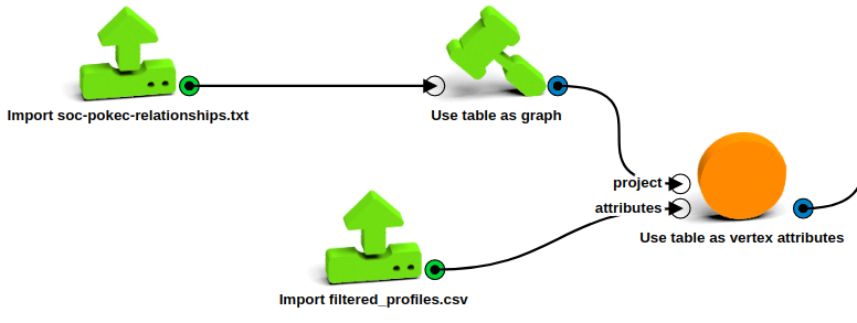
• First, let’s import the relationship data with a Import CSV operation. Choose the downloaded soc-pokec-relationships.txt file, change the delimiter to “\t”, set the ‘Columns in file’ parameter to Source,Destination (they come without a column name) and click on Run.
• The profiles dataset is previously filtered to make it easier to handle. To do it yourself drop all the columns except the 1st, 4rd, 5th, 6th, 7th and 8th and name them User_ID, Gender, Region, Last_Login, Registration and Age respectively. Filter out the observations whose Region attribute doesn’t contain ‘prievidza’. Transform the Last_Login and Registration attributes to days since last login and days since registration. Import the resulting dataset.

Build the graph

• Build the graph with the Use table as graph operation, connect it to the imported relationship data and link Source to Destination attributes. Check that you have 1.6M vertices with 30.6M edges.
• With the Use table as vertex attributes operation, join the graph with the profiles table imported. Use stringId for the vertex attribute and User_ID for the ID column.

Filter the vertices

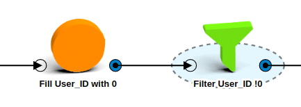
• Fill the missing User_ID values with 0 with a Fill vertex attributes with constant default values box.
• Filter out the vertices with User_ID = 0 using a Filter by attributes operation and setting the User_ID attribute as “!0”.

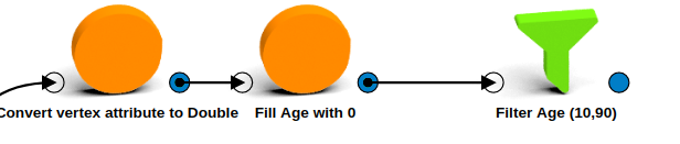
• Convert Age, Gender, Last_Login_Days, Registration_Days and User_ID attributes to Double.
• Our dataset comes with a default value of 0 for the users without age. In case any user does not have this default value, use a Fill vertex attributes with constant default values operation to fill it with 0s.
• Filter outliers, users with age below 10 or above 90 are more likely to be fake and we don’t want to use them for our prediction. We will go back to this point for the real prediction after we choose our method.

• Filter out disconnected vertices.
• Add a Find connected components operation to segment the vertices into components.
• With an Aggregate from segmentation box, aggregate the maximum size from the components to the vertices to differentiate which component each vertex belongs to.
• Filter out the vertices disconnected from the main component with a Filter by attributes box connected_components_size_max attribute greater than 10000.

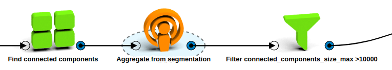
Check that you end up with 17777 vertices and 212368 edges.

Divide into train and test set

• To select a prediction model, we will use only the users that have a defined age attribute to be able to compare the age prediction with the real age value.
• Use a Split to train and test set to divide the age attribute into train and test with a test set ratio of 0.1 and a random seed of 1167456500 (to make this example reproducible).
• Let’s clean the working environment before we start building the models. Discard the vertex attributes Region and connected_components_size_max and the segmentation connected_components.

Model description

Now that we have a clean dataset divided into train and test set, we can sart building different models to predict the user’s age. In this example we will use three different models, evaluate them and pick the best one.

• The first model, we build a linear regression without any graph features, so we predict the age based on Gender, User_ID, Last_Login and Registration features.
• The second model, we predict the age as the average of the user neighbor’s age. In a graph, two vertices are neighbors if there is an edge that connects them.
• In the third model we build a linear regression to predict age according to some calculated graph features (degree, clustering coefficient, triangles) and the original non-graph features.
• For the final model, we assume that there are communities of connected users within the graph (e.g. a school community where users are connected with each other and have more or less the same age). Out of these communities, we take the one that has the lowest age variation and predict the age as the average of this community age.

We will use the training age set to build the models and with these models predict the test set age. Then, compare it with the real test set age values and choose the best model to use it with the previously separated users.

Linear regression with non-graph features prediction

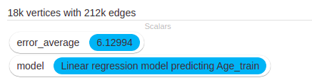
• Use a Train linear regression model operation to predict Age_train based on Gender, Last_Login_Days, Registration_Days and User_ID.
• Predict the age with a Predicth with model operation, change the prediction name to Age_prediction.
• Calculate the prediction error by deriving a vertex attribute and calculate the absolute difference between Age_prediction and Age_test with the following equation: ***Math.abs(Age_test
• Age_prediction)***.
• Find the Mean Absolute Error by computing the global error across vertices with a Aggregate vertex attribute globally operation.

Neighbor prediction

• With an Aggregate on neighbors operation, calculate the average of the neighbors Age_train attribute across all edges.
• Rename the newly calculated attribute to Age_prediction .
• Calculate the error of this prediction by copying the operations of the previous prediction.

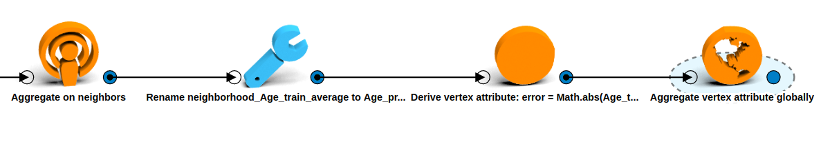
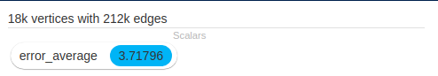
The resulting prediction average error is 3.71 years. It predicts the age for 17,556 nodes (98.75%), it leaves out those users whose neighbor’s don’t have a defined age attribute.

Linear regression with graph features prediction

Calculate attributes

• To build a regression model we need features that could be correlated with the user’s age. By doing some research (e.g. Inferring User Demographics and Social Strategies in Mobile Social Networks, A Study of Age and Gender seen through Mobile Phone Usage Patterns in Mexico) we determine that the following attributes might be correlated with the user’s age:
  • Degree: Number of connection the user has.
  • Gender triads: Gender proportion of the triangles the user belongs to (MMM, FMM, FFM, FFF). Triangle is a 3 pairwise connected vertices.
  • Clustering coefficient: Measurement of how closed are nodes clustered together. It shows how close are the vertex’s neighbors to become a clique.
  • Neighbor’s age: Average of the neighbor’s age as calculated in the first model.
  • Neighbor’s age variation: Variation of the connected user’s age.
  • Negihbor’s gender proportion: Proportion of male/female user’s connections.
• These attributes assume that the nature of the connection between users change with age, a reasonable proposition.
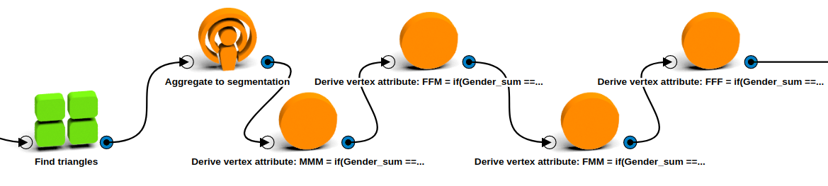
• Let’s start by calculating the Gender triads proportion.
• First, we need to group the users into triangles. We do this by using a Find triangles segmentation operation.
• With an Aggregate to segmentation operation, calculate the average of the gender in each triangle (1 is for males and 0 for females). This gives us the number of males in each triangle.
• In the triangles segmentation, derive 4 new vertex attributes, one for each type of triad possible. Calculate them with the following formulas:
  • MMM Triad: if(Gender_sum == 3.0) 1.0 else 0.0
  • FMM Triad: if(Gender_sum == 2.0) 1.0 else 0.0
  • FFM Triad: if(Gender_sum == 1.0) 1.0 else 0.0
  • FFF Triad: if(Gender_sum == 0.0) 1.0 else 0.0

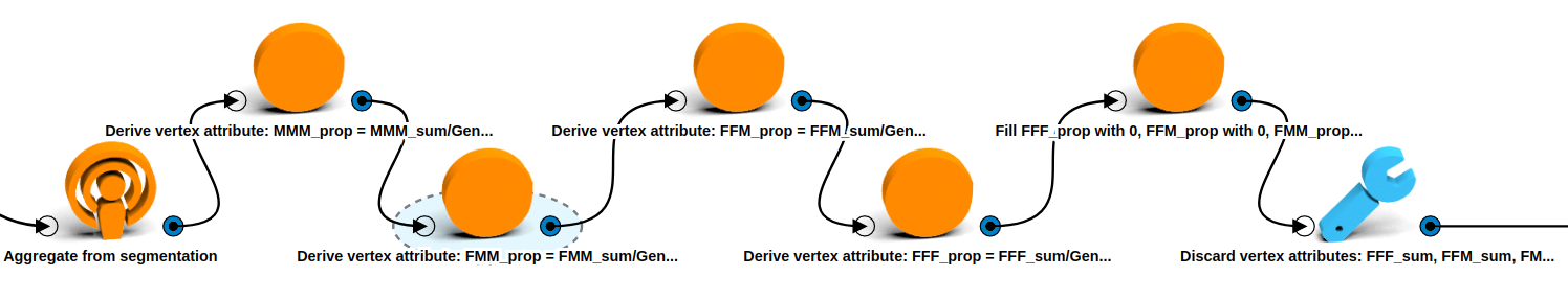
• Now we have to find the proportion of each triad over the total number of triads a user belongs to. Transfer the sum of each triad to the users with an Aggregate from segmentation operation, include also the count of the Gender_sum attribute to know how many triads the user belongs to.
• Derive 4 new vertex attributes corresponding of the proportion of each type of triad over the total number of triads that a user belongs to:
  • MMM_prop: MMM_sum/Gender_sum_count
  • FMM_prop: FMM_sum/Gender_sum_count
  • FFM_prop: FFM_sum/Gender_sum_count
  • FFF_prop: FFF_sum/Gender_sum_count
• It might be the case that there are some vertices without any triads, to avoid any error for those users, let’s Fill vertex attribute with constant 0 values for each gender triad proportion.
• Finally, let’s discard the unwanted vertex attributes, MMM_sum, FMM_sum, FFM_sum, FFF_sum, Gender_sum_count_.

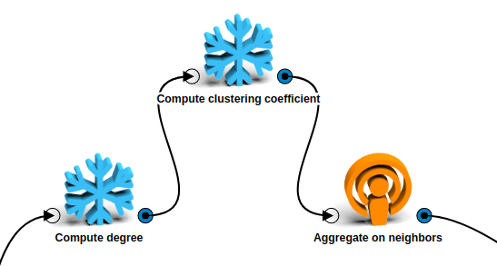
• Calculate the degree with a Compute degree operation taking all edges into consideration.
• Calculate the clustering coefficient with a Compute clustering coefficient operation.
• Finally, calculate the neighbor’s age average, age variation and gender proportion with a Aggregate on neighbors operation taking the average and standard deviation of the Age_train_ attribute and the average of the Gender attribute.

Estimate Age

• Now that we have all the features computed, we can go ahead and train a linear regression model with the Age_train attribute as target with a Build a Linear rergession model operation. Select all the attributes we previously calculated and Last_Login_Days, Registration_Days and Gender as Features.
• Let’s check our regression model results.
• From the T-values we can see that none of the gender triads were significant in the model, that is caused because they are codependant and using all of them cause perfect multicollinearity. When we take out the FFF_prop attribute they do become significant and positively correlated with age.
• The clustering coefficient is very significant and has a positive correlation with age, which means that older users have more contacts that know each other.
• The degree is also significant but with a negative relation with age, younger users tend to have more contacts.
• Neighbor’s age average is highly signficant and it has a direct relation with the user’s age.
• Neighbor’s age variation also has a positive correlation with the user’s age, older users tend to have more variation in their contact’s age.
• Neighbor’s gender proportion is negatively correlated, which means that younger users tend to have more male connections.
• Let’s predict our test set age. Use a Predict with model operation and set the prediction name to Age_prediction. Copy and paste the error calculating operations used for the other models.

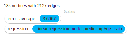
The calculated error goes down to 3.60 years, which is not a lot better than the simple attribute propagation. Let’s try a decision tree regression.

• Use a Train a decision tree regression model operation with the same parameters as the linar regression, predict the test set with another Predict with model box and find the average error as in the rest of the methods.

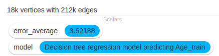
The decision tree error went down to 3.52 which is still not a big improvement.

Community prediction

Find Communities

• Divide the vertices into communities with a Find infocom communities box. This operation combines cliques (subgraphs where every vertex is connected) if they overlap sufficiently. Set the Edge required in cliques in both directions parameter to false. Leave the other parameters as they are.
• Open the new communities segmentation. There are 6K segments covering 13K vertices, which means around 5K vertices do not belong to any community. This means that they do not have overlapping cliques to merge. This would leave many users without an age prediction. Anyways let’s check how good the estimation using these communities would be.

Estimate Age

• LynxKite comes with an operation that predict an attribute based on the known values of the attribute on peers that belong to the same segments. This is the Predict attribute by viral modeling operation, it uses the segment with the lowest standard deviation to predict an attribute. Let’s use this operation on our communities segmentation and set the parameters as follows:
  • Target attribute: Age
  • Test set ratio: 0.1
  • Random seed: 1167456500 (same as the used before).
  • Maximal segment deviation: 3
  • Minimum number of defined attributes in segment: 3
  • Minimal ratio of defined attributes in a segment: 0.25
  • Iterations: 3
• In each iteration, the algorithm will calculate the age for each user that belongs to a segment that complies with the set parameters. In the next iteration it will use the newly computed age to estimate the age of the users which were not calculated before.
• After running, the algorithm predicted the age for 16785 vertices (94.4% of total users).
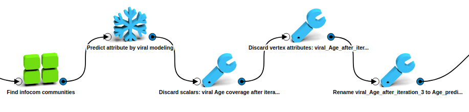
• To make sure that the algorithm is using the right test set to calculate the error, comparable with the rest of models, we need to compare the prediction with the original test set we previously separated. Let’s discard the unwanted attributes and scalars, rename the viral_Age_after_iteration_3 attribute to Age_prediction and re-compute the error as done in previous models. We confirm that the error is the same as the one found by viral modeling.

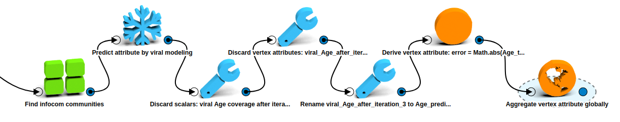
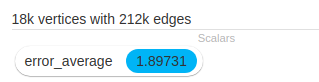
The error is 1.89 years but it doesn’t predict for outliers (users that only belong to a two person community).

Method selection

Out of the methods selected, the one with lower mean absolute error was the last one (viral modeling according to communities). The problem of this model is that it does not predict the age for every user, it leaves out the ones that are not part of a community. We can combine this model with the second one (neighbor’s average) to get a prediction for most users. For the remaining users, we can use the overall age average.

Real age prediction

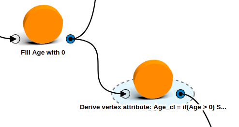
• Go back to before we filled the missing age attribute with 0s (before filtering the outliers). We need to predict the age for those users whose age is currently 0. First, let’s delete the 0s by deriving a new Age attribute with this function: if(Age > 0) Some(Age) else None.

• Now, let’s get the dataset ready for the prediction. Start with the communities prediction, copy and paste the community prediction operations without changing any of the parametes.

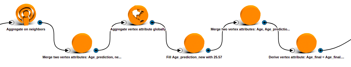
• Use an Aggregate on neighbors operation to find the second set of predictions. Compute the average of the Age attribute on neighbors. Merge both predictions into a single Age_prediction_new attribute with a Merge two vertex attributes operation.

• For the last users which don’t have a prediction yet we will use the overall age average.
• Calculate the age average across all users with an Aggregate vertex attribute globally operation and select the average of the Age attribute.
• With a Fill vertex attribute with constant default values operation, fill the newly calculated Age_predicted_new attribute with the age average value of 25,57.
• Combine the original Age attribute and the final prediction Age_predicted_new in a single Age_final attribute with a Merge two vertex attributes operation so that we have a single age per user. This will take the original age if the user has it and if not it will take the final prediction.
• We don’t really want the predicted user’s age to have decimal points, so let’s clear them out with a Derive vertex attribute operation to run Age_final.toInt.toDouble and save it again as Age_final.

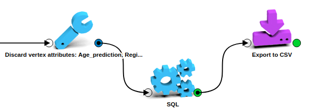
• Discard the unwanted vertex attributes (everyone except Age, Age_final, Gender and User_ID), pass it to a SQL1 box (without limit) and use a final Export to CSV box to download the results.

Results

We tackled a common data science problem of imputing missing data. We tried four different models and found that a combination of two of them would actually be the best approach to solve it. The final dataset has no missing data and is downloaded directly as a CSV file.