LynxKite for powerful graph data science on top of Neo4j

14 Oct 2020 — Andras Nemeth, CTO

If you already have a Neo4j database, then you have already completed a few important steps in your graph journey: you know how you want to model (some aspects of) your business as a graph, probably you are already using your data for ad-hoc graph queries, local investigations, or, maybe even in your operations!

But – just like you wouldn’t use an SQL database directly in table oriented data science – if you want to succeed in a complex, iterative graph data science project you need more than just a graph database.

In a classical, table oriented project you would use something like Pandas or Spark from Python, drop in some ML framework like PyTorch or use an integrated DS tool like RapidMiner or Dataiku. But whatever your choice of tool, you would work with snapshots of data and you would end up with a complex workflow of many interdependent operations.

If you have a serious graph project on your hand, however, you should turn to LynxKite! Now it’s made super easy with our new Neo4j connectors.

For the record, if you want to do graph data science but you do not have a graph DB yet, that’s also totally fine. You can use LynxKite directly to turn your traditional data into graphs. But this post is not about that.

Let’s now consider a simple but typical graph data science effort in detail. Take Neo4j’s Northwind dataset. (Just enter :play northwind-graph into your Neo4j browser and follow the instructions to get it.) This is a graph representing customers’ order histories. It contains nodes representing customers, orders, products, product categories and suppliers. What we want to achieve is identifying groups of products that are catering to similar “taste”, based on how often they were bought by the same customer.

Getting the data

First of all, let’s get our data into LynxKite! This is very simple using the new Neo4j import box:

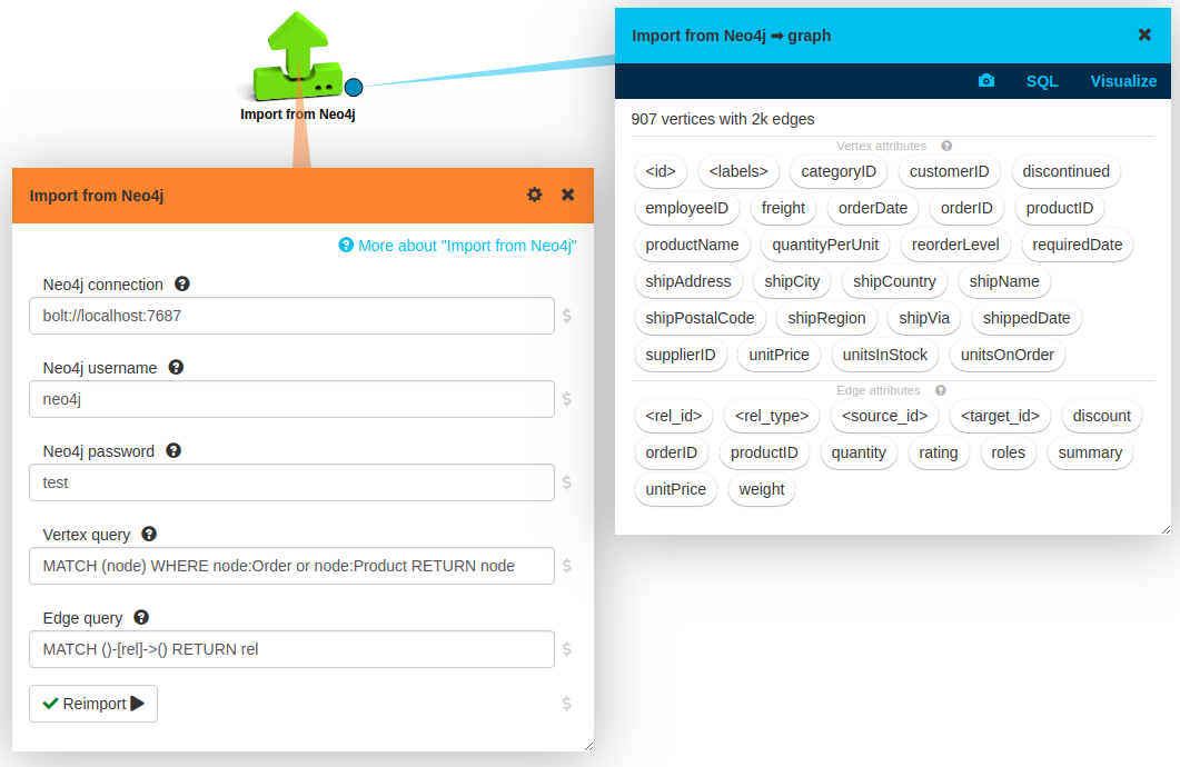
You just drop an Import from Neo4j box on your LynxKite workspace, set up your connection parameters, press Import, and you are good to go.

If you leave the default values for queries then all your data is imported. In this case we modified the node query by adding a WHERE clause: right now we are only interested in orders and products.

Here is a small sample of the imported graph:

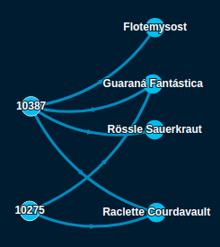
On the left, you can see two orders and on the right the ordered products.

Graph transformations

It is very rare that you just want to run a canned graph algorithm on a graph as it is available in your production systems. Very often you want some structural changes and you want the actual algorithms run on a modified graph.

It is important to note that these steps form an integral part of the data science project, very often we want to iterate on them a lot. In LynxKite, these steps are first class citizens in your analysis workflow. You can easily change the details and can easily rerun the whole downstream analysis. If you were to do this directly in a graph DB then you would have to go through painful cleanups and graph recreations in every iteration.

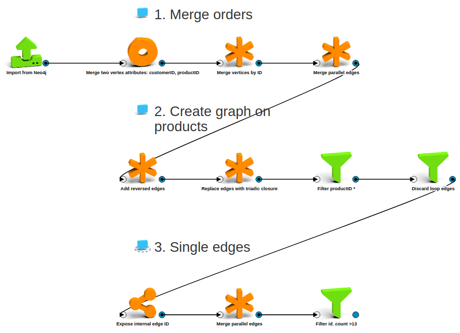
In our specific case, we want to go from an order - product bipartite graph to a graph on the products alone, where edges represent the number of customers that bought both connected products. We do the following transformation steps:

1. We merge orders by customer id: for this analysis, we do not care which products were bought in the same order, just the same customer matters.
2. We add reversed edges and then compute the triadic closure. With this, we end up with exactly the edges we want among the products, except we also create a bunch of loop edges for each product. So we remove those, and also we keep only nodes representing products, not (merged) orders.
3. Finally, we merge all parallel edges into single edges and keep the cardinality of the original parallel edges as an edge attribute. We also only keep edges representing frequent enough shared customers.

We can complete all above by dropping a few boxes on our workspace. Here is the full flow for graph transformations:

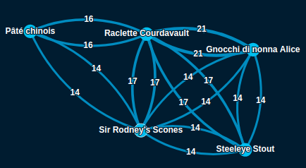
And here is a sample of the resulting graph:

Finding and labeling clusters

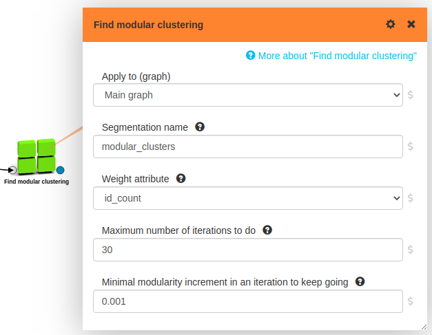
Now that we have the graph we want, running a clustering algorithm on it is trivial, we just drop in a Find modular clustering box:

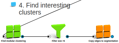
Well, we do tweak a bit afterwards: we remove very small clusters and we copy edges from products to product clusters so we can see how related the different clusters are to each other. Here is the full flow:

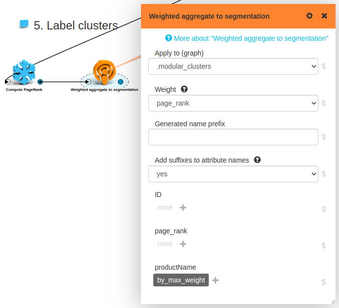
We are basically done, but let’s do one more cosmetic improvement! Let’s find for each cluster the most important product and use the name of that product as a label for our cluster. It’s easy: we just compute PageRank on the product graph and take the name of the highest PageRank product for all clusters:

Now it’s time to marvel at the result of our (not so) hard work! Here is a visualization with all the interesting, labeled clusters (right side), together with the members of one (on the left):

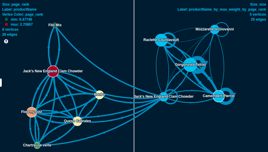
Interesting that almost all clusters are dominated by some kind of a cheese.. Always knew, cheese rocks!

Back to Neo4j

To close the loop, let’s get back the results of our analysis to the database! We need two simple preparatory steps. We give a nicer name to our aggregated label attribute, the one we want to see in the DB. Then we move it from the cluster to all its members. Finally, we just apply a Neo4j export box:

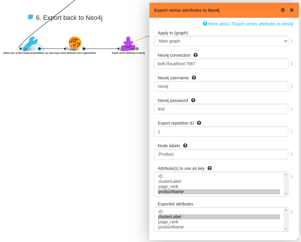
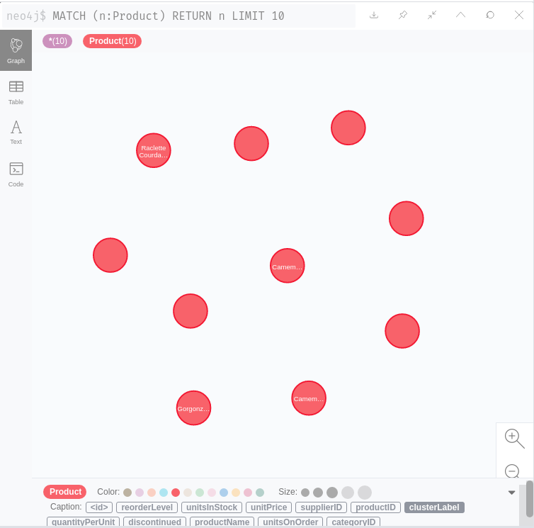
And indeed, the cluster labels show up in Neo4j as expected!

In this case, we wanted to export vertex attributes back to the DB, but it’s possible to do the same with edge attributes , or you can even push a complete graph to the DB.

All in code

Our experience is that iterative, explorative graph data science can be done more efficiently on a UI: it’s much easier to change things around, to inspect values and metadata at any point, no need to remember parameter names, etc. That said, some people prefer coding, and also, it’s the only reasonable way to go for automated, production deployment of data science pipelines.

For these cases we provide a powerful and simple Python API. Just for demonstration and without further explanation, see below the python code executing the full analysis detailed above.

import lynx.kite
lk = lynx.kite.LynxKite()

original = lk.importFromNeo4jNow(
    url='bolt://localhost:7687',
    username='neo4j',
    password='test',
    vertex_query='MATCH (node) WHERE node:Order or node:Product RETURN node')

users_and_products = (original
  .mergeTwoVertexAttributes(attr1='customerID', attr2='productID', name='ID')
  .mergeVerticesByAttribute(aggregate_productName='majority_100', key='ID', add_suffix='no')
  .mergeParallelEdges())

graph_on_products = (users_and_products
  .addReversedEdges()
  .replaceEdgesWithTriadicClosure()
  .filterByAttributes(filterva_productName='*')
  .discardLoopEdges())

single_edges = (graph_on_products
  .exposeInternalEdgeID()
  .mergeParallelEdges(aggregate_id='count')
  .filterByAttributes(filterea_id_count='>13'))

labeled_clusters = (single_edges
  .findModularClustering(weights='id_count')
  .filterByAttributes(apply_to_graph='.modular_clusters', filterva_size='>5')
  .copyEdgesToSegmentation(apply_to_graph='.modular_clusters')
  .computePageRank()
  .weightedAggregateToSegmentation(
      apply_to_graph='.modular_clusters',
      weight='page_rank',
      aggregate_productName='by_max_weight'))

(labeled_clusters
  .renameVertexAttributes(
      apply_to_graph='.modular_clusters',
      change_productName_by_max_weight_by_page_rank='clusterLabel',
      change_id='',
      change_size='')
  .copyVertexAttributesFromSegmentation(apply_to_graph='.modular_clusters', prefix='')
  .exportVertexAttributesToNeo4jNow(
      url='bolt://localhost:7687',
      username='neo4j',
      password='test',
      labels=':Product',
      keys='productName',
      to_export='clusterLabel'))

Recap

We performed above a simple but interesting analysis on the Northwind dataset. But the main point here is not about the concrete details of this analysis, nor the result. What we wanted to demonstrate is why even a fairly simple project needs steps and capabilities that are not possible or very cumbersome to do directly in a live, transactional graph database.

But we’ve come with good news! With our new connectors now it is super easy to use the free, open source LynxKite on top of your Neo4j instance for efficient and comfortable graph data science!

Try LynxKite Now